First Course Ding: Chapter 5

Stratification and post-stratification

Chapter 5 moves from completely randomized experiments to blocked and post-stratified designs. The Penn unemployment experiment is the real-data blocked example, and the later post-stratification section in the R script is simple enough to keep as explicit arithmetic.

from pathlib import Path

import matplotlib.pyplot as plt
import numpy as np
import pandas as pd

import crabbymetrics as cm

np.set_printoptions(precision=4, suppress=True)


data_dir = Path("../data/ding")

1 Penn Job-Training Data

penndata = pd.read_table(data_dir / "Penn46_ascii.txt", sep=r"\s+")
y = np.log(penndata["duration"].to_numpy(dtype=float))
z = penndata["treatment"].to_numpy(dtype=float)
block = penndata["quarter"].to_numpy()

unadjusted = cm.OLS()
unadjusted.fit(z[:, None], y)

block_dummies = pd.get_dummies(penndata["quarter"], drop_first=True, dtype=float)
blocked_design = np.column_stack([z, block_dummies.to_numpy(dtype=float)])
blocked = cm.OLS()
blocked.fit(blocked_design, y)


def stratified_diff(y, z, block):
    levels = np.unique(block)
    pieces = []
    for level in levels:
        idx = block == level
        zk = z[idx]
        yk = y[idx]
        pieces.append(
            {
                "weight": idx.mean(),
                "tau": yk[zk == 1.0].mean() - yk[zk == 0.0].mean(),
            }
        )
    out = pd.DataFrame(pieces)
    return float(np.dot(out["weight"], out["tau"]))


def neyman_sre(y, z, block):
    levels = np.unique(block)
    estimate = 0.0
    variance = 0.0
    for level in levels:
        idx = block == level
        zk = z[idx]
        yk = y[idx]
        weight = idx.mean()
        treated = zk == 1.0
        control = zk == 0.0
        tau_k = yk[treated].mean() - yk[control].mean()
        var_k = yk[treated].var(ddof=1) / treated.sum() + yk[control].var(ddof=1) / control.sum()
        estimate += weight * tau_k
        variance += (weight**2) * var_k
    return estimate, variance


stratified_estimate, stratified_variance = neyman_sre(y, z, block)


summary_table = pd.DataFrame(
    {
        "estimate": [
            unadjusted.summary()["coef"][0],
            blocked.summary()["coef"][0],
            stratified_estimate,
        ],
        "se_hc1": [
            unadjusted.summary(vcov="hc1")["coef_se"][0],
            blocked.summary(vcov="hc1")["coef_se"][0],
            np.sqrt(stratified_variance),
        ],
    },
    index=["Unadjusted OLS", "Blocked OLS", "Weighted block mean"],
)
summary_table

	estimate	se_hc1
Unadjusted OLS	-0.079601	0.030275
Blocked OLS	-0.091458	0.030603
Weighted block mean	-0.089906	0.030798

2 Fisher Test Within Blocks

rng = np.random.default_rng(5)
observed_stat = stratified_diff(y, z, block)
null_draws = np.zeros(1000)

for rep in range(null_draws.size):
    z_perm = z.copy()
    for level in np.unique(block):
        idx = np.flatnonzero(block == level)
        z_perm[idx] = rng.permutation(z_perm[idx])
    null_draws[rep] = stratified_diff(y, z_perm, block)

lower_tail = np.mean(null_draws <= observed_stat)
two_sided = np.mean(np.abs(null_draws) >= abs(observed_stat))
pd.DataFrame(
    {
        "observed_stratified_stat": [observed_stat],
        "one_sided_lower_pvalue": [lower_tail],
        "two_sided_pvalue": [two_sided],
    }
)

	observed_stratified_stat	one_sided_lower_pvalue	two_sided_pvalue
0	-0.089906	0.0	0.002

fig, ax = plt.subplots(figsize=(6, 4))
ax.hist(null_draws, bins=40, alpha=0.75)
ax.axvline(observed_stat, color="black", linestyle="--", linewidth=2.0)
ax.set_xlabel("Stratified difference in means")
ax.set_ylabel("Count")
ax.set_title("Randomization distribution under blockwise permutations")
fig.tight_layout()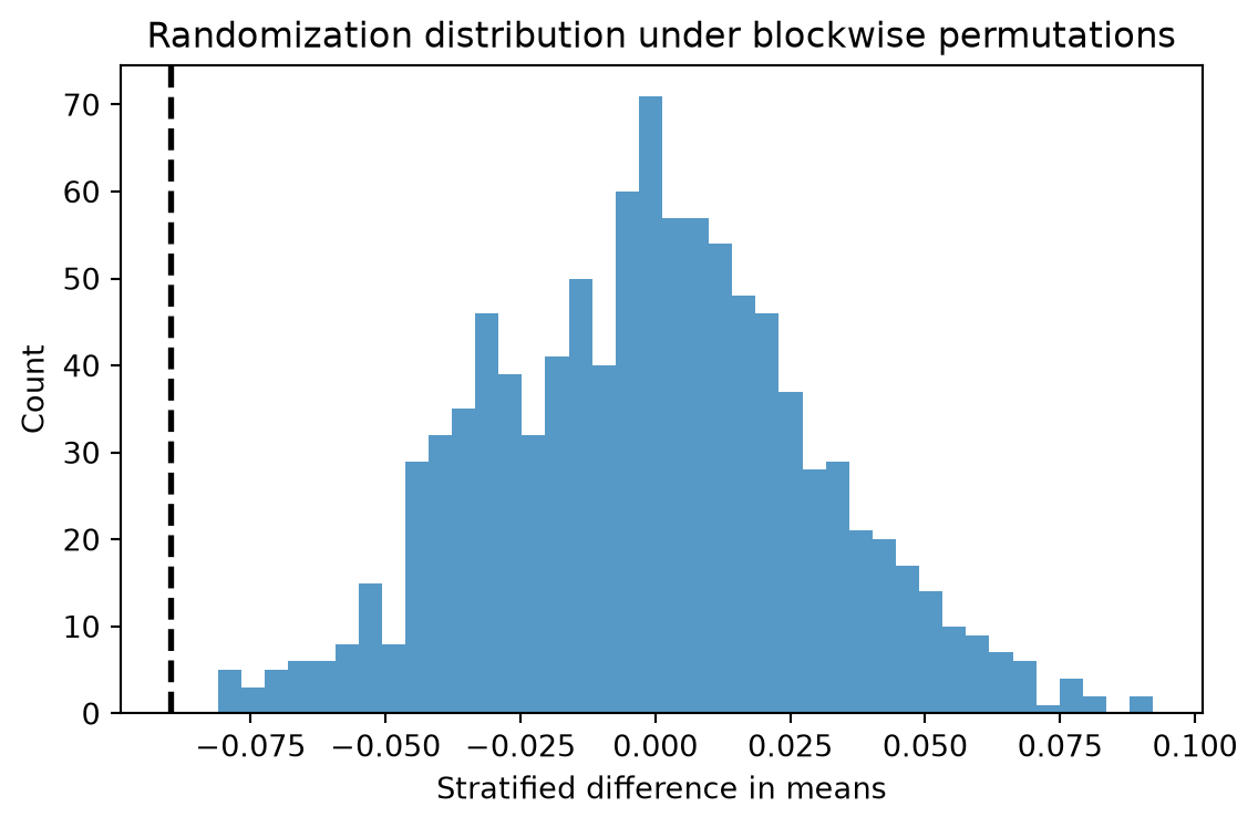

3 Post-Stratification Arithmetic

The source script also has a small two-stratum binary-outcome example. It is useful because there is no modeling hidden inside it: each stratum contributes its own risk difference and binomial variance, then the overall post-stratified estimate weights by stratum size.

post_counts = pd.DataFrame(
    [
        ("stratum 1", 1, 98, 8),
        ("stratum 1", 0, 115, 5),
        ("stratum 2", 1, 76, 22),
        ("stratum 2", 0, 69, 16),
    ],
    columns=["stratum", "treated", "success", "failure"],
)
post_counts["n"] = post_counts["success"] + post_counts["failure"]
post_counts["rate"] = post_counts["success"] / post_counts["n"]
post_counts["binom_var"] = post_counts["rate"] * (1.0 - post_counts["rate"]) / post_counts["n"]

pieces = []
for stratum, df in post_counts.groupby("stratum", sort=False):
    treated_row = df.loc[df["treated"] == 1].iloc[0]
    control_row = df.loc[df["treated"] == 0].iloc[0]
    pieces.append(
        {
            "name": stratum,
            "n": df["n"].sum(),
            "estimate": treated_row["rate"] - control_row["rate"],
            "variance": treated_row["binom_var"] + control_row["binom_var"],
        }
    )

stratum_table = pd.DataFrame(pieces)
weights = stratum_table["n"] / stratum_table["n"].sum()
post_est = float(np.dot(weights, stratum_table["estimate"]))
post_var = float(np.dot(weights**2, stratum_table["variance"]))

treated_total = post_counts.loc[post_counts["treated"] == 1, ["success", "n"]].sum()
control_total = post_counts.loc[post_counts["treated"] == 0, ["success", "n"]].sum()
treated_rate = treated_total["success"] / treated_total["n"]
control_rate = control_total["success"] / control_total["n"]
crude_est = treated_rate - control_rate
crude_var = (
    treated_rate * (1.0 - treated_rate) / treated_total["n"]
    + control_rate * (1.0 - control_rate) / control_total["n"]
)

pd.DataFrame(
    {
        "estimate": [
            *stratum_table["estimate"].to_list(),
            post_est,
            crude_est,
        ],
        "se": [
            *np.sqrt(stratum_table["variance"]).to_list(),
            np.sqrt(post_var),
            np.sqrt(crude_var),
        ],
    },
    index=[*stratum_table["name"].to_list(), "post-stratified", "crude"],
)

	estimate	se
stratum 1	-0.033805	0.031480
stratum 2	-0.036255	0.059784
post-stratified	-0.034901	0.031908
crude	-0.044620	0.032609

4 Takeaway

The chapter’s logic survives the translation almost unchanged:

• the design determines which permutations are admissible
• conditioning on strata can tighten the estimator
• the blocked estimator is just a weighted average of within-block contrasts
• post-stratification is the same weighted-average idea applied after observing a discrete covariate partition