MatrixCompletion Example

Low-rank counterfactual completion for treated panel cells

MatrixCompletion fits observed untreated cells and predicts treated-cell counterfactuals. The public panel API is the same as the other high-level panel estimators: fit(Y, W) where Y is an N × T outcome matrix and W is a same-shaped absorbing-treatment indicator.

This example uses a genuinely low-rank untreated panel, adds unit and time effects, masks treated cells through W, and asks MatrixCompletion to fill the counterfactual surface.

Objective and RMSE histories refer to the same post-update iterate. An objective increase no longer satisfies the convergence check. summary(include_matrices=False) omits the four large arrays completed, low_rank, counterfactual, and treatment_effect; diagnostics, effects summaries, and one-dimensional arrays remain available. The default still returns independent owned matrices.

For incomplete panels, use NaNs or fit(Y, W, observed=mask). The missing-outcome example explains the estimator-specific fitting rules.

1 Simulate A Low-Rank Panel

import matplotlib.pyplot as plt
import numpy as np

from crabbymetrics import MatrixCompletion

np.set_printoptions(precision=4, suppress=True)

rng = np.random.default_rng(4402)

n_units = 52
n_periods = 30
time = np.arange(n_periods)
rank = 2

unit_effects = rng.normal(scale=0.4, size=n_units)
time_effects = 0.05 * time + 0.4 * np.sin(time / 4.0)
loadings = rng.normal(size=(n_units, rank))
factors = np.vstack(
    [
        np.sin(np.linspace(0.0, 2.5 * np.pi, n_periods)),
        np.cos(np.linspace(0.0, 1.5 * np.pi, n_periods)),
    ]
)

Y0 = unit_effects[:, None] + time_effects[None, :] + loadings @ factors
Y = Y0 + rng.normal(scale=0.08, size=Y0.shape)
W = np.zeros_like(Y)

treated_units = np.arange(8)
cohort_starts = np.r_[np.repeat(18, 4), np.repeat(23, 4)]
for unit, start in zip(treated_units, cohort_starts):
    W[unit, start:] = 1.0
    Y[unit, start:] += 0.9 + 0.04 * np.arange(n_periods - start)

true_att = float((Y - Y0)[W == 1].mean())
print("Y shape:", Y.shape)
print("treated cells:", int(W.sum()))
print("true ATT:", round(true_att, 4))

Y shape: (52, 30)
treated cells: 76
true ATT: 1.085

2 Fit Matrix Completion

model = MatrixCompletion(
    lambda_fraction=0.20,
    fit_unit_effects=True,
    fit_time_effects=True,
    max_iterations=400,
    tolerance=1e-6,
)
model.fit(Y, W)
summary = model.summary()

print("estimated ATT:", round(float(summary["att"]), 4))
print("lambda_l:", round(float(summary["lambda_l"]), 4))
print(
    "fit diagnostics:",
    {key: summary[key] for key in ["converged", "iterations", "termination_reason", "objective"]},
)
print("final observed-cell RMSE:", round(float(summary["history_rmse"][-1]), 4))

estimated ATT: 1.1784
lambda_l: 0.0088
fit diagnostics: {'converged': True, 'iterations': 7, 'termination_reason': 'Relative objective tolerance reached', 'objective': 0.36268185281652116}
final observed-cell RMSE: 0.2593

completed = np.asarray(summary["completed"])
counterfactual = np.asarray(summary["counterfactual"])
treatment_effect = np.asarray(summary["treatment_effect"])

fig, axes = plt.subplots(1, 3, figsize=(13, 4.0), constrained_layout=True)

for ax, matrix, title in [
    (axes[0], Y, "Observed Y"),
    (axes[1], counterfactual, "Counterfactual Surface"),
    (axes[2], treatment_effect, "Observed - Counterfactual"),
]:
    im = ax.imshow(matrix, aspect="auto", cmap="viridis")
    ax.set_title(title)
    ax.set_xlabel("Period")
    ax.set_ylabel("Unit")
    fig.colorbar(im, ax=ax, shrink=0.78)

plt.show()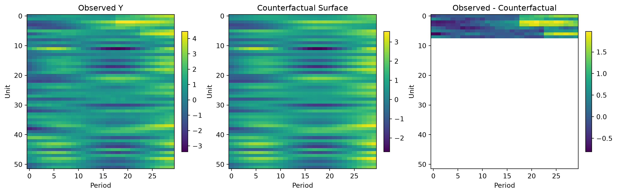

summary() also returns the low-rank component, singular values, event-study summaries, and group means. The important contract is that the estimator owns the panel bookkeeping: users supply matrices, not hand-built donor lists or long data frames.