Masked matrix completion, available-case SDID and overlap-specific ridge
Missing outcomes are not zeros. Pass an N\times T outcome matrix containing NaN, or supply fit(Y, W, observed=mask) to ignore selected entries. The three estimators use the same observation mask but different fitting rules.
Estimator
What a missing outcome changes
Matrix completion
Removes that cell from the low-rank fitting loss.
Synthetic DID
Removes its contribution from both the numerator and denominator of a weighted average.
Horizontal ridge
Selects donors available at prediction time and fits on their jointly observed pre-periods.
W is a known treatment schedule, separate from outcome availability. When adoption dates are known, construct W[i, t] = (t >= adoption[i]), even where Y[i, t] is missing. Unknown treatment is not automatically coded as untreated.
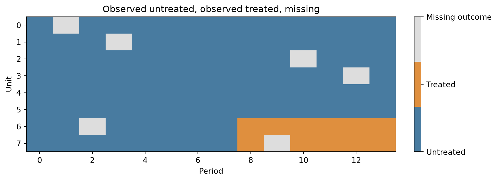
A panel with holes
This example has six donors, two treated units and a constant treatment effect of 1.25. It removes donor and treated outcomes both before and after adoption.
Code
import numpy as npimport pandas as pdimport matplotlib.pyplot as pltfrom matplotlib.colors import ListedColormapfrom IPython.display import displayimport crabbymetrics as cmrng = np.random.default_rng(941)time = np.arange(14)donors = rng.normal(size=(6, 1)) + rng.normal(size=(6, 2)) @ np.vstack( [np.sin(time /3), time /8])baseline =0.3* donors[0] +0.7* donors[3] +0.4Y = np.vstack([donors, baseline -0.15, baseline +0.15])W = np.zeros_like(Y)W[6:, 8:] =1Y +=1.25* Wobserved = np.ones(Y.shape, dtype=bool)for i, t in [(0, 1), (1, 3), (2, 10), (3, 12), (6, 2), (7, 9)]: observed[i, t] =False
All three ATTs target the observed treated cells. Matrix completion and ridge average their observed post-treatment prediction errors. SDID also subtracts its time-weighted pre-treatment gap. SDID’s displayed counterfactual uses the unit-fit intercept, so averaging its diagnostic effect matrix is not the SDID ATT. Missing treated outcomes have no reported effect, even when a counterfactual can be predicted there.
Matrix completion: mask the loss
Let R_{it} indicate an observed outcome and define \Omega=\{(i,t):R_{it}=1,\ W_{it}=0\}. The objective is
The same mask is used in fixed-effect updates, the singular-value-thresholding step, penalty scaling and convergence diagnostics. Neither missing entries nor treated outcomes enter the loss. Low-rank predictions can cover both.
Each unit and period must have an observed untreated outcome. With both fixed effects enabled, the observed-untreated unit–period graph must be connected. These are support checks, not a guarantee that a particular low-rank model fits.
SDID: normalize over available observations
For donor weights \omega, the synthetic outcome at period t is
The unit-weight fit compares this with the observed treated-cohort pre-period mean, using a free intercept and the existing squared-weight penalty. Time weights use the analogous available-period average for each donor. Their target is that donor’s observed post-period mean, weighted by the number of observed treated outcomes at each post-period and renormalized over the donor’s observed periods.
Rows without an observed target and columns without training observations are excluded. Missing cells enter neither sum. A zero available-weight denominator is an error, not a zero synthetic outcome.
This is an available-case extension of SDID. Unlike the complete-panel quadratic problem, the denominators depend on the weights, so the objective can be nonconvex. The implementation profiles out the intercept and uses simplex-projected gradient descent with backtracking, initialized uniformly. It reports its objective and projected-gradient residual and fails if the iteration budget expires without stationarity. Complete panels retain the existing active-set quadratic solver.
Within a cohort, the ATT averages observed post-treatment gaps using the number of observed treated cells per period, then subtracts the fitted time-weighted pre-gap. Cohorts are combined using their observed treated post-cell counts. Default penalties use adjacent observed donor pre-period differences; gaps are not bridged when estimating the noise scale.
Code
diagnostics = models["Synthetic DID"].summary()["missing_diagnostics"]rows = []for d in diagnostics:for kind in ["unit", "time"]: rows.append({"Cohort": d["cohort"], "Weights": kind,"Iterations": d[f"{kind}_iterations"],"Objective": d[f"{kind}_objective"],"Gradient residual": d[f"{kind}_projected_gradient"]})display(pd.DataFrame(rows))
Cohort
Weights
Iterations
Objective
Gradient residual
0
8
unit
67
0.034660
7.976549e-09
1
8
time
7
0.999626
0.000000e+00
Ridge: missing outcomes can also be missing predictors
Horizontal ridge uses donor outcomes as regressors. Dropping a missing response does not resolve a missing donor regressor. For each cohort and prediction period:
Select donors observed at that period with some pre-period overlap.
Select pre-periods with an observed treated-cohort mean and observations for every selected donor.
Fit ordinary ridge on that observed design, with an unpenalized intercept, and predict from the selected donors.
Periods with identical donor availability reuse the same fitted model. No donor feature is filled with zero or its mean. If an observed treated post-period has no donor/training overlap, the fit raises an explicit error. This rule can still run out of common pre-periods in a very sparse panel; it does not manufacture a full design by filling missing regressors.
summary()["overlap_models"] identifies the donors, training periods and coefficients used for each prediction. When a cohort needs multiple models, its legacy single cohort_coef/cohort_intercepts row is NaN rather than displaying one model as if it applied to every period.
Code
overlap = models["Horizontal ridge"].summary()["overlap_models"]display(pd.DataFrame([{key: value for key, value in model.items()if key !="coef"} for model in overlap]))
cohort
periods
donors
training_periods
intercept
0
8
[0, 2, 4, 5, 6, 7, 8, 9, 11, 13]
[0, 1, 2, 3, 4, 5]
[0, 2, 4, 5, 6, 7]
1.058420
1
8
[1]
[1, 2, 3, 4, 5]
[0, 1, 2, 4, 5, 6, 7]
0.986261
2
8
[3]
[0, 2, 3, 4, 5]
[0, 2, 3, 4, 5, 6, 7]
0.993076
3
8
[10]
[0, 1, 3, 4, 5]
[0, 2, 4, 5, 6, 7]
0.878841
4
8
[12]
[0, 1, 2, 4, 5]
[0, 2, 4, 5, 6, 7]
1.119325
What the checks establish
The test suite compares masked MC against observed-only two-way FE least squares, ridge against independently constructed NumPy regressions, and SDID against SciPy optimization of the same normalized objectives. It also checks low-rank recovery, complete-panel parity, missing-value placeholder invariance, and that changing treated post outcomes cannot change the fitted counterfactual.
Handling missing entries removes a computational obstacle; it does not identify effects for selectively unobserved outcomes. Interpreting the observed-cell ATT still requires the estimator’s counterfactual assumptions and a suitable observation process.