Credit Markets: alternative counterfactual models

CS-DID, SDID, matrix completion, horizontal ridge and partially pooled staggered synthetic control

Noack and Costello (2024) study property rights and fishing mortality. This comparison extends the Credit Markets replication with Callaway–Sant’Anna DID and four synthetic-control or outcome-model estimators, on the same sample. CS-DID reports both the dynamic/event-study aggregate and the simple treated-unit-year aggregate. The latter matches the averaging weights used by the other counterfactual summaries.

Results JSON · Quarto source · Code and environment · Archive index

import sys
from pathlib import Path

import crabbymetrics as cm
import matplotlib.pyplot as plt

ROOT = next(
    p
    for p in [Path.cwd(), *Path.cwd().parents]
    if (p / "templates/full_archive").exists()
)
OUT = ROOT / "analyses/credit-markets/crabbymetrics"
sys.path.insert(0, str(OUT / "templates"))

from fit_crabby import fit_one
from report_support import (
    adoption_plot,
    event_plot,
    prepare_panel,
    publish_results,
    results,
    scalar_plot,
    show_table,
)

data, Y, W, baseline = prepare_panel()

Data and sample

The outcome is asinh(ffmsy): fishing mortality relative to the maximum-sustainable-yield benchmark. Treatment is EEZ/property-rights adoption, coded 0 or 1. Units are stock–country pairs; time is annual, 1960–2012. There are no additional covariates in this specification.

All models use the existing 723-unit × 53-year panel, comprising 529 treated units in 15 adoption cohorts and 194 never-treated units. The 21 units already treated in 1960 are excluded. No further observations are dropped. The panel contains 38,319 observations and 17,811 treated unit-years, across 47 countries.

The outcome is divided by 1.3291711871762193, the original full-source sample SD before exclusions. It is not demeaned. Adoption is the first treated year within a unit; event time is year minus adoption year.

preview = data[["time", "d", "g", "y"]].copy()
preview["time"] += 1959
preview["g"] = preview["g"].where(preview["g"].eq(0), preview["g"] + 1959)
preview = preview.rename(
    columns={
        "time": "Year",
        "d": "Treatment",
        "g": "Adoption year",
        "y": "Outcome / SD",
    }
)
preview.head()

	Year	Treatment	Adoption year	Outcome / SD
0	1960	0	1977	4.041307
1	1961	0	1977	4.111993
2	1962	0	1977	4.079477
3	1963	0	1977	4.122737
4	1964	0	1977	4.160667

adoption_plot(W)
plt.show()

The adoption plot shows a seeded sample of 100 units. Estimation uses all 723.

Estimators

Estimator	Counterfactual model and settings
CS-DID	Python csdid.ATTgt, doubly robust estimation with no covariates, not-yet-treated controls and universal cohort-specific year −1 reference. aggte(typec="dynamic") supplies the event path and equal-event-time scalar; aggte(typec="simple") supplies the matched treated-unit-year scalar.
SDID	crabbymetrics.SyntheticDID: donor and pre-period weights fitted separately for each adoption cohort; default data-dependent penalties.
Matrix completion	crabbymetrics.MatrixCompletion: unit effects, time effects and a nuclear-norm-regularized low-rank component, fitted to all untreated cells. lambda_fraction=0.25; exact SVD; objective tolerance 10^{-12}.
Horizontal ridge	crabbymetrics.HorizontalPanelRidge: regress each cohort’s pre-treatment mean on the never-treated outcome histories, with an intercept and ridge penalty 1. Predict using contemporaneous donor outcomes.
Multisynth (individual)	time_cohort=FALSE: 529 unit-level synthetic controls fitted jointly, with partial pooling. nu=NULL, lambda=0, fixed-effect adjustment and nonnegative donor weights.
Multisynth (cohort-averaged)	time_cohort=TRUE: 15 cohort-level synthetic controls fitted jointly, with partial pooling and the same other settings.

CS-DID uses never-treated units plus other cohorts untreated in both comparison periods. SDID, horizontal ridge and multisynth use the 194 never-treated donors. Matrix completion also uses untreated observations from units that adopt later. The three crabbymetrics estimators follow the staggered-panel vignette, with a tighter matrix-completion stopping tolerance.

Callaway–Sant’Anna DID

CS-DID estimates one ATT for each adoption cohort and calendar year. This fit uses est_method="dr", control_group="notyettreated", xformla="y ~ 1", anticipation=0 and base_period="universal". With no covariates, each group-time point estimate is the cohort’s mean outcome change from its year −1 minus the corresponding change among never-treated and eligible not-yet-treated units. The focal cohort is excluded from its own controls, and eligibility requires remaining untreated through both the baseline and comparison year.

from fit_csdid import fit_csdid

csdid = fit_csdid(data)
from csdid_aggregations import aggregation_table

show_table(aggregation_table(csdid))

CS-DID: -0.3929733704; country-clustered SE: 0.0933063436
Checks: {'max_group_time_vs_direct_did_difference': 4.718447854656915e-16, 'max_dynamic_if_vs_direct_if_difference': 7.105427357601002e-15, 'independent_country_cluster_se': 0.09330634356069892, 'country_cluster_se_difference': 0.0, 'scalar_vs_equal_event_average': np.float64(0.0), 'simple_vs_treated_cell_average': 0.0, 'group_time_cells': 795, 'post_treatment_cells': 439, 'treated_unit_years': 17811}

Aggregation	Estimate (SDs)	SE	95% CI
Equal post-event times	-0.3930	0.0933	[-0.5759, -0.2101]
Equal treated unit-years	-0.4901	0.0781	[-0.6432, -0.3369]
Cohort-size-weighted post-period means	-0.4944	0.0779	[-0.6470, -0.3418]

The same not-yet-treated group-time estimates support three distinct scalar aggregations, as defined in the aggregation documentation:

• Dynamic (typec="dynamic"): average cohort effects using cohort-size weights within each event time, then average the 46 post-event estimates equally over years 0–45. balance_e=None leaves cohort composition free to change with the horizon.
• Simple (typec="simple"): weight every available post-treatment cohort–year ATT by that cohort’s size. On this complete balanced panel, this is exactly the 17,811 treated-unit-year average used by Sun–Abraham and the other counterfactual summaries. It is the matched-aggregation CS-DID row in the main table and figure.
• Group (typec="group"): first average post-treatment years within each cohort, then average those cohort means using cohort-size weights. This gives each treated unit equal total weight regardless of its number of observed post-treatment years. It does not match the treated-unit-year target here.

Let n_g be cohort size, T_g its observed post-period count, and \bar\tau_g=T_g^{-1}\sum_{t\geq g}\widehat{ATT}(g,t). Then

\widehat\theta_{simple}= \frac{\sum_g n_g T_g\bar\tau_g}{\sum_g n_g T_g}, \qquad \widehat\theta_{group}= \frac{\sum_g n_g\bar\tau_g}{\sum_g n_g}.

For event time e, let G_e contain cohorts observed at that exposure. The dynamic scalar is

\widehat\theta_{dynamic}=\frac{1}{46}\sum_{e=0}^{45} \frac{\sum_{g\in G_e}n_g\widehat{ATT}(g,g+e)}{\sum_{g\in G_e}n_g}.

The group and simple weights differ because T_g ranges from 3 to 46 years. The two main CS-DID rows therefore are not separate model fits: they use identical controls, observations and group-time effects, with different aggregation weights. The group summary is retained in this section and JSON as an additional diagnostic, not substituted for the matched-cell row.

All three standard errors use analytical influence functions, summed within the 47 country clusters (clustervar="cluster", bstrap=False, cband=False). They include uncertainty in estimated cohort shares. Independent calculations reproduce each scalar, its influence function and its standard error. Intervals are pointwise 95% normal intervals, not simultaneous bands.

SDID

This implementation handles staggered adoption by fitting a separate block-adoption SDID for each of the 15 cohorts. Each fit contains that cohort’s treated units and the 194 never-treated donors, split into pre/post periods at the cohort’s adoption date. Other adoption cohorts are excluded from its donor pool, including units not yet treated at that date.

Donor weights match the cohort’s mean pre-treatment outcome history. Pre-period weights match the donors’ average post-treatment outcomes using their pre-treatment observations. Both sets of weights are nonnegative and sum to one, with intercepts and the regularization settings below. The cohort ATT is the mean post-treatment treated–synthetic gap minus the time-weighted pre-treatment gap. Cohort ATTs are then weighted by treated-unit count times observed post-period count, yielding the same 17,811-cell target. There is no cross-cohort partial-pooling parameter. See the pinned implementation.

sdid = fit_one("SDID", cm.SyntheticDID(), {}, Y, W)

SDID -0.5028172865517654 seconds 0.07 diagnostics {'converged': True, 'pre_rmse': 0.0909946390628935}

Matrix completion

mc_settings = {
    "lambda_fraction": 0.25,
    "max_iterations": 1000,
    "tolerance": 1e-12,
    "fit_unit_effects": True,
    "fit_time_effects": True,
    "svd_method": "exact",
}
mc = fit_one("Matrix completion", cm.MatrixCompletion(**mc_settings), mc_settings, Y, W)

Matrix completion -0.5108673993931916 seconds 0.1 diagnostics {'converged': True, 'iterations': 44, 'termination_reason': 'Relative objective tolerance reached'}

Horizontal ridge

ridge = fit_one(
    "Horizontal ridge", cm.HorizontalPanelRidge(1.0), {"penalty": 1.0}, Y, W
)

Horizontal ridge 0.03214054573252869 seconds 0.15 diagnostics {'pre_rmse': 0.016141633743993137}

Partially pooled staggered synthetic control

Two R augsynth specifications are reported on the same sample:

• Individual-unit fits (time_cohort=FALSE): one donor-weight vector for each of the 529 treated units, fitted jointly to balance individual and pooled pre-treatment outcomes.
• Cohort-averaged fits (time_cohort=TRUE): one donor-weight vector for each of the 15 adoption cohorts, fitted jointly to balance cohort-mean and pooled pre-treatment outcomes. This uses cohort-mean histories, like SDID and horizontal ridge, while retaining cross-cohort partial pooling.

These are different fitting objectives, not merely two ways to average a single set of fitted effects. Both reported ATTs use the same 17,811 treated-unit-year weights, with fixedeff=TRUE, scm=TRUE and lambda=0. Each fit selects its own shared pooling parameter using nu=NULL.

The horizon is set to n_leads=46, covering event years 0–45 wherever observed, with n_lags=50 using all available pre-treatment history. This preserves all 17,811 treated unit-years. The default three-year post horizon would change the target. At the specified full horizon, the package’s donor-eligibility rule leaves exactly the same 194 never-treated donors for every adoption cohort; the fitted donor masks are checked directly.

from report_support import multisynth_comparison, run_multisynth

multisynth = run_multisynth()
multisynth_individual = run_multisynth(individual=True)
show_table(multisynth_comparison([multisynth_individual, multisynth]), digits=5)

Multisynth fit	time_cohort	Weight vectors	ATT (SDs)	Shared ν	λ
Individual-unit	FALSE	529	-0.35737	0.15164	0
Cohort-averaged	TRUE	15	-0.47334	0.60511	0

The cohort-averaged R call is shown below. The individual-unit call changes time_cohort to FALSE; the source bundle includes both executable scripts.

fit <- multisynth(
  y ~ d, stock_id, time, panel,
  n_leads = 46, n_lags = 50,
  nu = NULL, lambda = 0,
  fixedeff = TRUE, scm = TRUE, time_cohort = TRUE,
  eps_abs = 1e-6, eps_rel = 1e-6
)
effect <- predict(fit, att = TRUE)

Pooling and tuning parameters

Each multisynth specification uses one shared partial-pooling parameter \nu: 0.15163794 for the 529 individual-unit fits and 0.60511294 for the 15 cohort-averaged fits. Neither selects \nu separately by cohort. In the implemented objective, \nu=0 weights only separate fit imbalance and \nu=1 weights only pooled imbalance, with package-specific normalization of both terms.

With nu=NULL, the package first fits separate synthetic controls and sets \nu to its ratio of pooled to average separate-fit imbalance. This is a data-derived default, not cross-validation. Both realized values are reported above and repeated in the cohort table below. The weight-regularization parameter is \lambda=0; this is distinct from \nu, and no ridge augmentation is requested.

SDID and horizontal ridge still fit cohort-mean histories independently, with no cross-cohort partial-pooling parameter. Matrix completion estimates a shared low-rank structure jointly, but does not have a multisynth-style \nu.

Estimator	Pooling used in these fits	Pooling parameter	Regularization
CS-DID	Group-time DID contrasts	N/A	None in this intercept-only specification
SDID	Separate cohort-mean fits; no cross-cohort coupling	N/A	Cohort-specific \zeta_\omega and \zeta_\lambda, shown below
Horizontal ridge	Separate cohort-mean fits; no cross-cohort coupling	N/A	Ridge penalty 1 for every cohort
Multisynth (individual)	Jointly fitted unit-level weights; individual and pooled balance	Shared \nu=0.15163794	Weight penalty \lambda=0
Multisynth (cohort-averaged)	Jointly fitted cohort-level weights; cohort and pooled balance	Shared \nu=0.60511294	Weight penalty \lambda=0
Matrix completion	One shared low-rank matrix fitted jointly to all untreated cells	No separate \nu	Nuclear-norm penalty lambda_l=0.0010985526453507334, from lambda_fraction=0.25

Cohort-specific settings

All synthetic-control fits use 194 never-treated donors. The table reports actual tuning values in outcome-SD units. SDID uses its data-dependent defaults: \zeta_{\omega,g}=(N_g T_{\mathrm{post},g})^{1/4}\widehat\sigma_g and \zeta_{\lambda,g}=10^{-6}\widehat\sigma_g, where \widehat\sigma_g is computed from donor pre-treatment first differences. Both multisynth specifications’ shared \nu values and common \lambda are repeated by cohort for reference; horizontal ridge’s penalty is 1 throughout.

from report_support import show_cohort_tuning

tuning_models, _, _ = results()
show_cohort_tuning(tuning_models)

Adoption year	Treated units	Cohort ν (shared)	Individual ν (shared)	SDID ζω	SDID ζλ	Multisynth λ
1967	11	0.60511294	0.15163794	1.5834	3.338504e-07	0
1969	2	0.60511294	0.15163794	1.0334	3.374035e-07	0
1971	1	0.60511294	0.15163794	0.953616	3.745944e-07	0
1976	10	0.60511294	0.15163794	1.6631	3.792000e-07	0
1977	255	0.60511294	0.15163794	3.70602	3.786142e-07	0
1978	81	0.60511294	0.15163794	2.74681	3.764353e-07	0
1979	46	0.60511294	0.15163794	2.34099	3.722547e-07	0
1980	7	0.60511294	0.15163794	1.43572	3.682697e-07	0
1982	4	0.60511294	0.15163794	1.21294	3.634825e-07	0
1983	82	0.60511294	0.15163794	2.5404	3.607182e-07	0
1984	1	0.60511294	0.15163794	0.841576	3.626552e-07	0
1995	15	0.60511294	0.15163794	1.47577	3.640646e-07	0
2000	1	0.60511294	0.15163794	0.677793	3.569530e-07	0
2005	12	0.60511294	0.15163794	1.11444	3.560313e-07	0
2010	1	0.60511294	0.15163794	0.461718	3.508298e-07	0

The results JSON includes explicit partial_pooling metadata for every estimator and a cohort_tuning record for each adoption cohort. A null parameter for the other methods means not applicable, not an unreported fitted value.

Controls, estimands and the CS-DID difference

The calendar panel is balanced: every one of the 723 units is observed in all 53 years. No additional covariates enter this specification (xformla="y ~ 1" for CS-DID). Unit/time fixed effects, lagged-outcome histories, learned donor weights and low-rank factors are parts of the respective estimators, not an added common covariate vector. The outcome scaling and eligible observations are identical across rows.

Method	Comparison information
CS-DID	Never-treated units plus eligible not-yet-treated units; controls are untreated in both comparison periods
Sun–Abraham	Never-treated reference group in this saturated fit
SDID, horizontal ridge, both multisynth fits	Never-treated donor units
BJS / did2s and matrix completion	All untreated observations, including pre-adoption observations of eventually treated units
Static and dynamic TWFE	Regression comparisons can involve already-treated units; neither is simply a never-treated/not-yet-treated design

The following audit reruns CS-DID on the identical sample, changing only the control group and aggregation. Both use the universal period −1 baseline, no covariates, and the same country clustering. Intervals are 95% analytical influence-function intervals.

controls	aggregation	estimate	se	lower	upper
nevertreated	Equal treated cells	-0.5138	0.0759	-0.6626	-0.3650
nevertreated	Equal post-event times	-0.4130	0.0922	-0.5937	-0.2322
notyettreated	Equal treated cells	-0.4901	0.0781	-0.6432	-0.3369
notyettreated	Equal post-event times	-0.3930	0.0933	-0.5759	-0.2101

With treated-cell weights, changing from never-treated to not-yet-treated controls moves CS-DID from −0.5138 to −0.4901. With equal-event-time weights, the same control change moves it from −0.4130 to −0.3930. Holding not-yet-treated controls fixed, changing aggregation instead moves the estimate by 0.0971 SD. Thus most of the earlier plotted separation came from weighting, not the choice of controls. The revised main comparison displays both CS-DID weighting rules. The never-treated, treated-cell CS-DID point estimate matches Sun–Abraham here, although their reported covariance calculations differ.

The event-time panel is not composition-balanced, despite the balanced calendar panel: event year 0 includes 529 treated units, whereas event year 45 includes only 11. Equal-event-time averaging gives these two event years equal weight; treated-cell averaging does not. No horizon-balancing restriction is applied.

These rows therefore do not all estimate the same scalar target. In particular, static TWFE is a coefficient benchmark, and dynamic TWFE’s aggregated coefficients need not equal a clean treated-cell ATT under effect heterogeneity. Identical final averaging weights do not remove event-study contamination. The alternative estimators also use different identifying restrictions on untreated outcomes.

Aggregate estimates

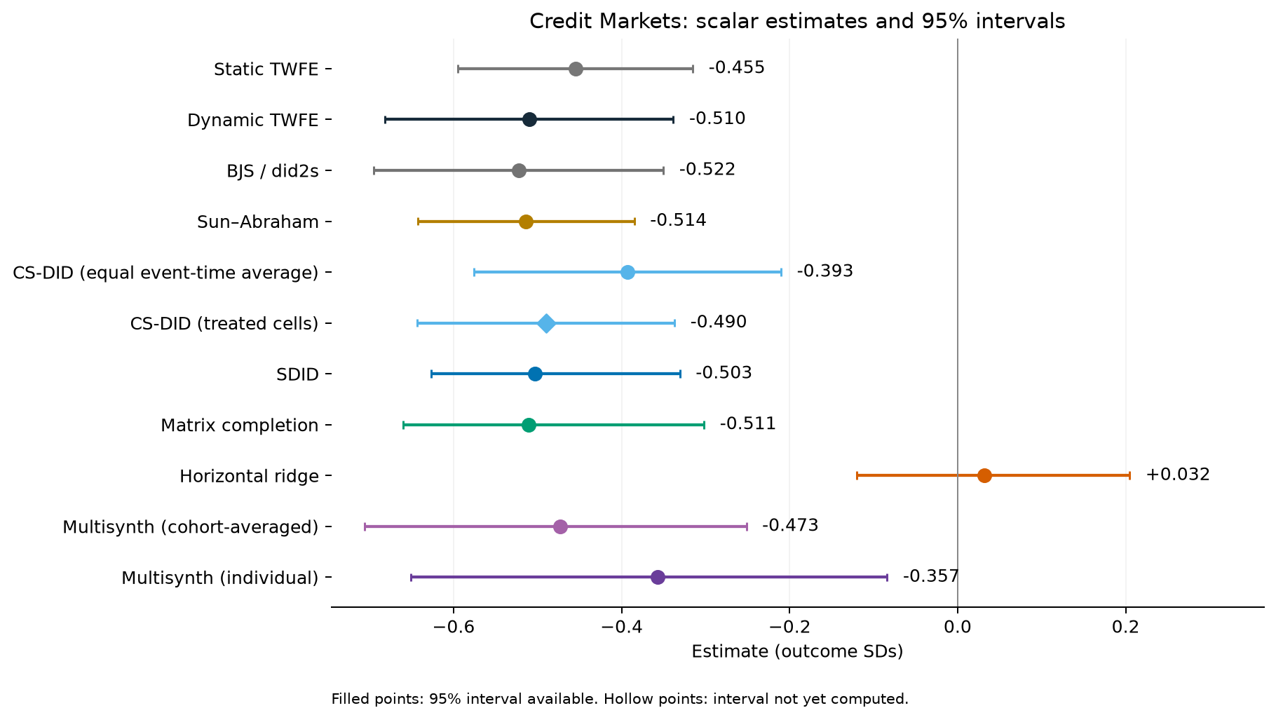
Two CS-DID summaries are shown: equal event years 0–45 and equal treated unit-years. The other dynamic and counterfactual summaries average effects over 17,811 treated unit-years, giving earlier cohorts more weight because they contribute more post-treatment observations. Static TWFE is its regression coefficient. These scalar weighting rules differ; none is Peter’s original equal-weight event-years 0–20 summary.

models, spec, estimates = results()
from report_support import estimate_rows

show_table(estimate_rows(estimates))
scalar_plot(estimates)
plt.show()

Estimator	Estimate (SDs)	95% CI	Aggregation
Static TWFE	-0.4550	[-0.5947, -0.3152]	Coefficient
Dynamic TWFE	-0.5098	[-0.6813, -0.3383]	Treated cells
BJS / did2s	-0.5225	[-0.6948, -0.3501]	Treated cells
Sun–Abraham	-0.5138	[-0.6428, -0.3849]	Treated cells
CS-DID	-0.3930	[-0.5759, -0.2101]	Equal event-time
CS-DID (treated cells)	-0.4901	[-0.6432, -0.3369]	Treated cells
SDID	-0.5028	[-0.6262, -0.3306]	Treated cells
Matrix completion	-0.5109	[-0.6602, -0.3018]	Treated cells
Horizontal ridge	0.0321	[-0.1202, 0.2047]	Treated cells
Multisynth (cohort-averaged)	-0.4733	[-0.7055, -0.2514]	Treated cells
Multisynth (individual)	-0.3574	[-0.6508, -0.0838]	Treated cells

SDID and matrix completion are close to BJS and Sun–Abraham. Horizontal ridge gives a small positive estimate. All estimates use the same sample and outcome scale.

For both multisynth fits, the reported scalar weights each observed treated unit-year equally. The package’s final predict() row instead averages individual post-treatment means equally, or cohort post-treatment means weighted by cohort size, without the additional post-period-count weighting; the JSON records those alternative summaries separately. The plotted event path and the reported scalar use the existing archive target weights.

Both multisynth specifications remain in this comparison: individual −0.3574 SD; cohort-averaged −0.4733 SD. The earlier −0.4495 SD came from separate ridge-augmented cohort fits, a different estimator not included in these two multisynth rows.

The scalar figure displays 95% intervals for all eleven summaries. Regression rows retain country-clustered CRV1 intervals; both CS-DID summaries use country-clustered influence-function intervals. SDID, matrix completion and horizontal ridge use 999 whole-country pairs-bootstrap refits, recomputing weights, data-dependent tuning and cohort shares while holding the source outcome-SD denominator fixed; their intervals are bootstrap percentiles. Both multisynth fits use 9,999 country-clustered Mammen wild-bootstrap draws from the package’s fixed-weight prediction procedure, with no jackknife or QP refits. A common multiplier is applied to all units within each of the 47 countries, and every draw is aggregated over the same 17,811 treated cells. These are basic bootstrap intervals conditional on fitted weights, pooling/tuning and the observed design—not full-refit pairs-bootstrap intervals. Their 95% ranges are [−0.7055, −0.2514] for cohort fits and [−0.6508, −0.0838] for individual fits.

Event studies

Counterfactual models

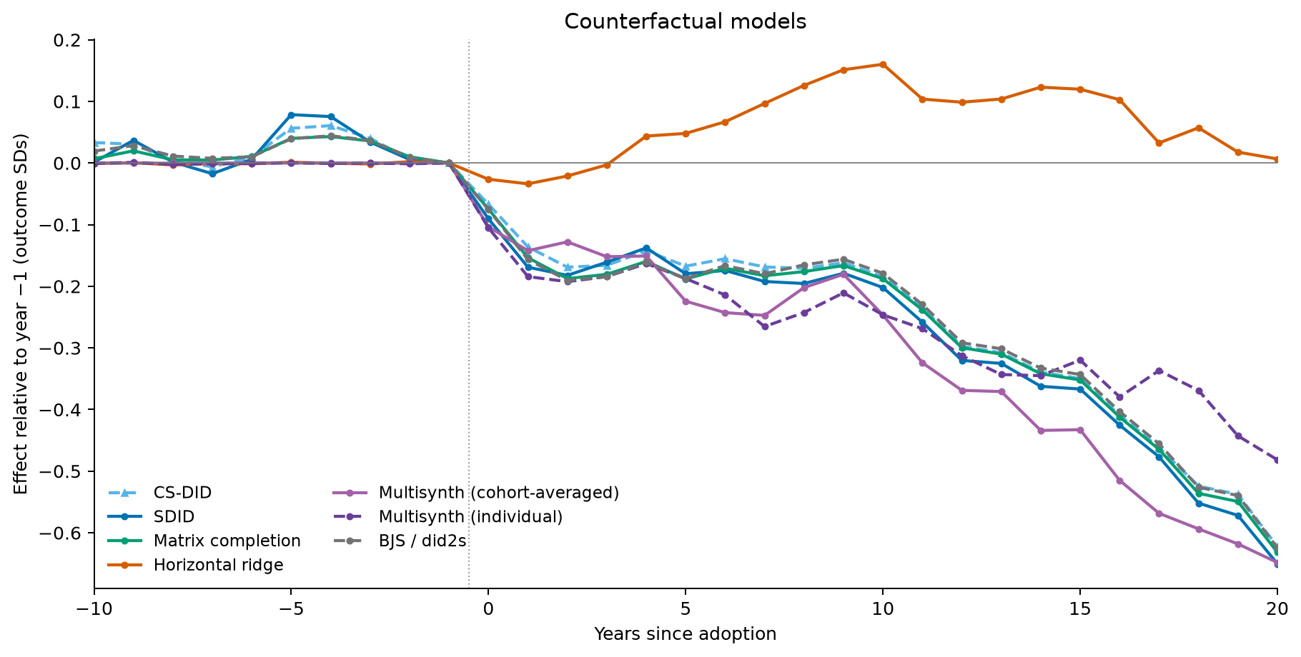
Each curve is centered on its own event-time −1 value, as in the crabbymetrics example. This is a plotting normalization only: the aggregate estimates above are not shifted. Curves show years −10 through 20; the JSON includes the complete paths and the number of contributing units at each event time.

For SDID, the package’s event summary is the raw synthetic-control gap, whereas its scalar ATT also subtracts a time-weighted pre-treatment gap. The SDID path below applies that subtraction within each cohort before aggregation. Its uncentered post-period average therefore equals the package’s ATT. Both raw and corrected gaps are retained in the JSON.

event_plot(models, spec)
plt.show()

Individual versus cohort-averaged multisynth

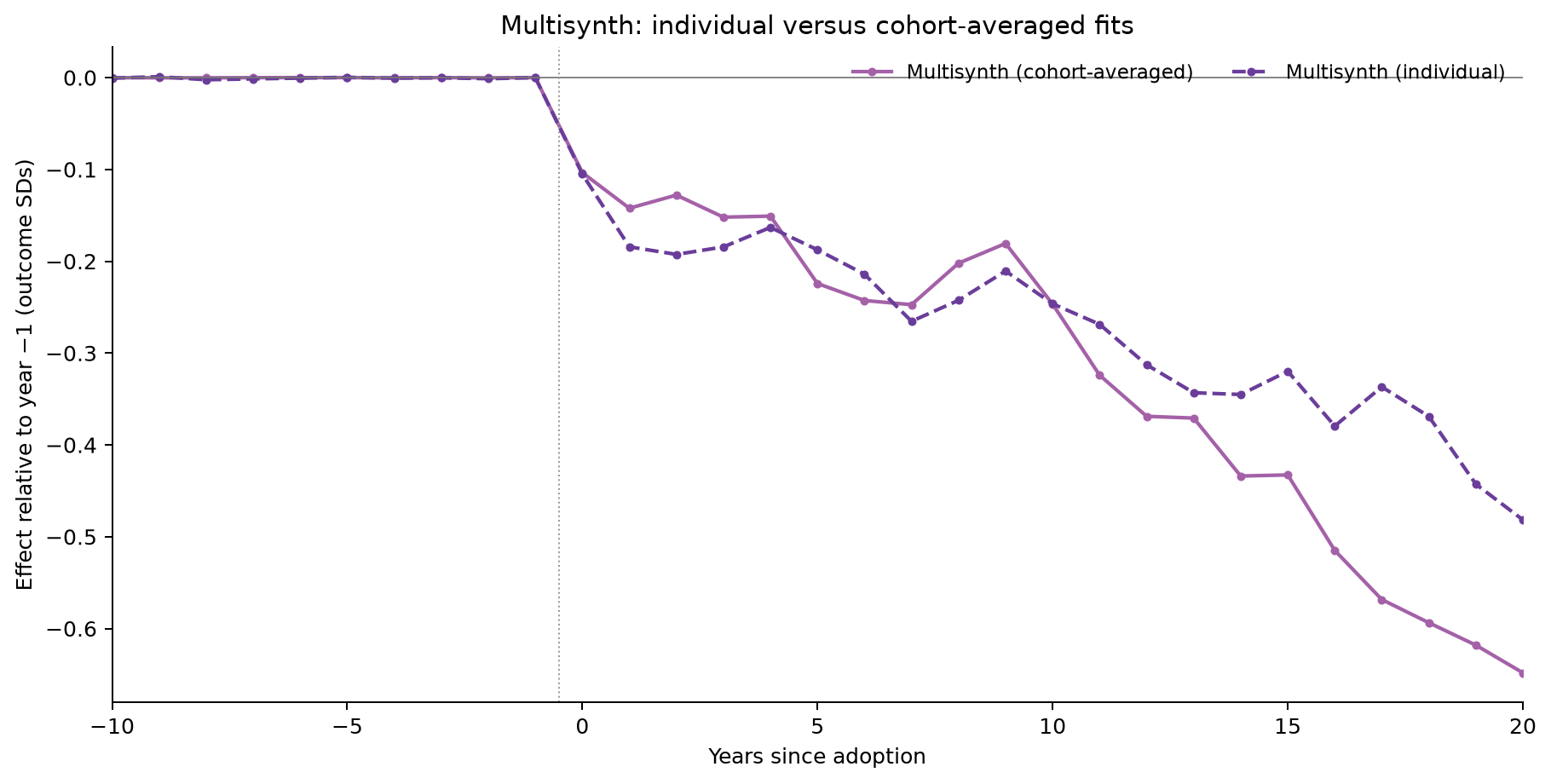
This isolates the two multisynth event paths. Both are centered at their own event-time −1 value for plotting only; their reported scalar ATTs are not recentered. The JSON includes both full event paths and both fits’ cohort-level summaries.

event_plot(models, spec, only_multisynth=True)
plt.show()

Regression benchmarks

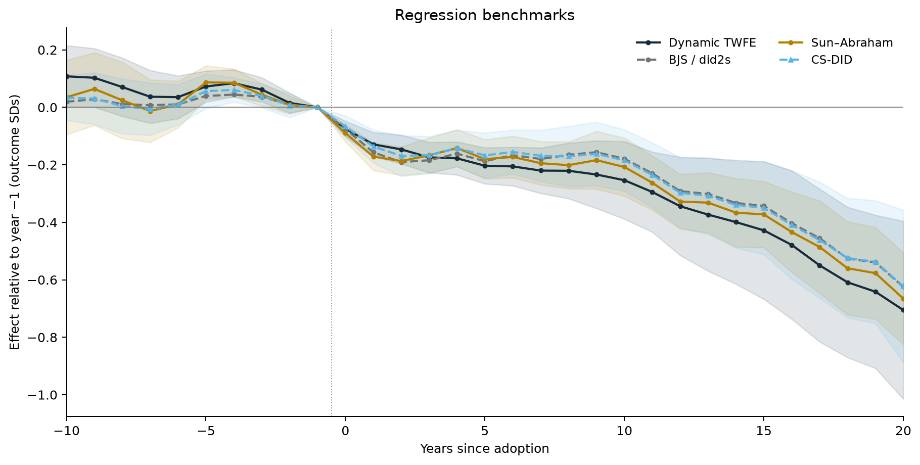
These are dynamic TWFE, BJS, Sun–Abraham and CS-DID on the identical sample. Shaded bands are country-clustered 95% pointwise intervals for TWFE, Sun–Abraham and CS-DID, using each estimator’s reported covariance calculation. CS-DID now uses not-yet-treated controls, while Sun–Abraham retains its earlier specification. BJS is centered on its estimated period −1 gap and shown as a point-estimate path. CS-DID uses dashed lines and triangle markers.

event_plot(models, spec, matrix=False)
plt.show()

Numerical checks

from validate_models import validate_models

checks = validate_models(Y, W, models)

• An independent closed-form calculation reproduces horizontal ridge to within 9\times10^{-11} SD.
• All 795 CS-DID group-time estimates match direct two-period DID contrasts to within 7\times10^{-16} SD. All 17,811 treated cells remain available; the dynamic scalar averages post-event times equally, while the simple scalar weights all treated cells equally. Independent influence functions, including cohort-share uncertainty, reproduce the dynamic, simple and group aggregates and country-clustered standard errors.
• Increasing SDID’s optimization budget from 1,000 to 5,000 iterations leaves the ATT unchanged.
• Matrix completion converges after 44 iterations at the reported tolerance. Tightening it from 10^{-12} to 10^{-14} changes the ATT by less than 1.6\times10^{-6} SD.
• Aggregation checks recover each scalar from its event path: equal post-event weights for CS-DID dynamic; treated-unit-year weights for CS-DID simple and the other new estimators. No treated cells are omitted.
• Multisynth’s event-time estimates agree with predict(fit, att=TRUE). A separate calendar-time reconstruction from the fitted weights and fixed-effect adjustment reproduces the reported treated-cell average. Solver statuses and balance diagnostics are included in the JSON.
• The 15-cohort multisynth fit uses the unmodified package’s native matrix construction. The 529-unit fit uses a call-scoped sparse construction of the identical optimization matrix; a four-unit check matches the unmodified package’s weights and predictions within 10^{-12}. All solver calls converge. Both scalar estimates independently match their calendar-time reconstructions.

exported = publish_results(models, spec, estimates)
print("Saved credit-markets-counterfactuals-results.json")
print("crabbymetrics:", sdid["crabbymetrics"])
print("augsynth:", multisynth["augsynth"])
print("csdid:", csdid["package"]["csdid"])

Saved credit-markets-counterfactuals-results.json
crabbymetrics: 0.9.1
augsynth: 0.2.0
csdid: 0.4.2

Reproduction and downloads

The source uses Python csdid 0.4.2 with drdid 1.1.6, crabbymetrics 0.9.1 from commit 896ceaf, and R augsynth 0.2.0 from commit 7e70072. uv add csdid updates the project environment and lockfile. All code and environment files are in the reproduction bundle. The source data stay in the existing local archive.

QUARTO_PYTHON=.venv/bin/python quarto render \
  analyses/credit-markets/crabbymetrics/credit-markets-counterfactuals.qmd

• Scalar estimates: PNG · PDF.
• Counterfactual event studies: PNG · PDF.
• Multisynth comparison: PNG · PDF.
• Regression event studies: PNG · PDF.
• Machine-readable results, including cohort diagnostics, settings, event paths and validation results.