---
title: "A Survey of Reinforcement Learning for Economics"
author: "Pranjal Rawat, Georgetown University"
date: "March 2026"
bibliography: refs.bib
jupyter: python3
format:
html:
toc: true
toc-depth: 3
number-sections: true
code-fold: true
code-summary: "Show code"
code-tools: true
code-overflow: wrap
execute:
echo: true
warning: false
message: false
cache: true
---
```{python}
#| label: setup
#| include: false
from pathlib import Path
import sys
for candidate in [Path.cwd(), Path.cwd() / "manuscript", Path.cwd().parent / "manuscript"]:
if candidate.exists():
sys.path.insert(0, str(candidate))
from quarto_helpers import display_image, display_tex_table, run_artifact
```
# Introduction {#section:intro}
This survey (re)introduces reinforcement learning to researchers studying sequential decision problems. I review the theoretical connections between dynamic programming and reinforcement learning, demonstrating how value iteration, Q-learning, and policy gradient methods are common solution methods to the same class of optimization problems. I then examine applications across several domains, including control problems, pricing and inventory management; structural economic models with high-dimensional state spaces; strategic games in which multi-agent algorithms compute equilibria under imperfect information; bandit problems in which economic structure yields tighter regret bounds; and preference learning. The exposition combines formal theory, practical applications and computational illustration.
Both dynamic programming and reinforcement learning solve the Bellman equation; they differ in the information requirements and the way in which the solution is refined. First, dynamic programming requires knowledge of the transition in the environment and the reward function which allows the reduction of the average Bellman error, reinforcement learning estimates value functions only from sampled transitions (observed sets of state, action, reward, next-state) which only allows reduction of the sampled Bellman error *at that state-action pair*. This allows us to improve policies in domains where it is easier to build a simulator than specify the model of the environment and rewards e.g. board games, physics simulators for robots. Second, dynamic programming makes a "breadth-first" (across all states and actions) update of the solution at each sweep, while reinforcement learning makes a "incremental" (only for the current state and action) update; this greatly reduces the computational burden and enhances scalability.
Reduction of average Bellman errors gives dynamic programming a geometric rate of convergence to the optimal solution, while the incremental updates and reduction of sampled Bellman errors, when combined with "sufficient exploration" of the state-action space, gives reinforcement learning only sublinear convergence guarantees. This is however, quite sufficient in practice, the scalability attained by only sampling transitions and making incremental updates more than makes up for the slower rates of convergence (and brittleness). These approximation methods sacrifice theoretical guarantees. RL algorithms lack the convergence assurances of exact dynamic programming. They exhibit sensitivity to hyperparameters and initialization. They can converge to suboptimal policies without diagnostic indication. This survey presents reinforcement learning as a computationally flexible framework while acknowledging its methodological limitations.
Theory in reinforcement learning trails empirical success, often by years; convergence guarantees, sample complexity bounds, and approximation error characterizations typically arrive after practitioners have demonstrated that an algorithm works. The theoretical insights that eventually follow tend to be deep and structural, and the empirical frontier is itself a productive research frontier. Experiments are brittle, conducted on benchmark environments that are stylized approximations of deployment settings. These benchmarks nonetheless serve a critical coordination function, aligning research effort, enabling reproducible comparison, and exposing failure modes that motivate new theory. Details matter disproportionately in reinforcement learning; small implementation choices can determine whether an algorithm converges or diverges, and the practice of releasing code and documenting hyperparameters, seeds, and preprocessing has proven essential to progress.
This survey focuses on less-surveyed intersections between reinforcement learning and applied decision-making, including the shared theoretical foundations, structural estimation, strategic interaction, bandit problems with domain structure, preference learning, and causal inference. Algorithmic collusion, in which independent pricing algorithms learn to sustain supra-competitive prices [@Calvano2020], is treated in a companion thesis chapter [@Rawat2026collusion] and omitted here. Reinforcement learning and deep learning methods for solving macroeconomic models with heterogeneous agents constitute a growing literature with dedicated methodological treatments [@AtashbarShi2022], [@MaliarMaliarWinant2021], and [@FernandezVillaverdeNunoPerla2024]. Portfolio optimization, optimal execution, and asset pricing via reinforcement learning form a large body of work surveyed comprehensively elsewhere [@HamblyXuYang2023]. The inverse problem of inferring preferences from observed behavior using inverse reinforcement learning and structural estimation is treated in a companion survey [@RustRawat2026].
The survey addresses the forward problem, that is, computing optimal policies given a known or simulated environment. Chapter 1 traces the parallel historical development of dynamic programming and reinforcement learning. Chapter 2 develops unified theory connecting planning and learning. Chapters 3 and 4 apply reinforcement learning to control problems and applied models. Chapter 5 examines strategic games. Chapter 6 addresses bandit problems. Chapter 7 discusses reinforcement learning from human feedback. Chapter 8 connects reinforcement learning to causal inference. Chapter 9 concludes.
# Two Cultures of Sequential Decision-Making {#section:language}
Two intellectual traditions both study sequential decision-making under uncertainty, but they descend from different intellectual traditions. The first is fundamentally an *inference culture*. Its central task is to understand the world. A "model" in this tradition is a specification of preferences, beliefs, constraints, and an equilibrium concept. The RL tradition is instead a *control culture*. Its central task is to act in the world. An RL researcher's "model" is a transition kernel $P(s'|s,a)$ and a reward function $r(s,a)$. These are different mathematical objects serving different scientific purposes.
The inference tradition concentrates its effort on specifying and estimating the objective function and the law of motion that governs the environment. The entire structural econometrics enterprise (demand estimation, dynamic discrete choice) is devoted to recovering these primitives from data, and the optimal policy is a byproduct that falls out once the primitives have been identified. The control tradition inverts this emphasis. Engineers typically take the objective and the dynamics as given (the cost function is specified, the plant physics are known or measurable) and focus on whether the optimal policy can be computed, approximated, and deployed under real-time and robustness constraints. The entire controls enterprise (PID, LQR, MPC, RL) is about computing and implementing the policy under different assumptions about what the agent knows and what it can compute.
The two cultures maintain different relationships with data. Econometricians work primarily with observational data, where endogeneity is the central obstacle; agents sort, markets clear, and unobservables correlate with the variables of interest. Identification, the question of whether the data can distinguish the true model from observationally equivalent alternatives, is the defining challenge, and it disciplines every modeling choice (functional forms, equilibrium definitions, instrumental variables, regression discontinuities, natural experiments). RL researchers have traditionally enjoyed what might be called *simulator omnipotence*. They own the data-generating process, can inject arbitrary variation through exploration policies, and can generate millions of on-policy rollouts at negligible marginal cost. Their binding constraint is computational (can the algorithm converge before the compute budget runs out?) rather than statistical (is the estimator consistent given the endogeneity structure of the data?). This asymmetry shapes everything downstream, from what counts as a valid result to what the word "model" means. To an econometrician, a model is a set of falsifiable restrictions on the joint distribution of observables and primitives. To an RL researcher, a model is a simulator you can call.
The two fields also share a vocabulary ("agent," "learning," "model," "policy") whose meanings diverge in ways that create persistent confusion. The subsections below provide a systematic translation.
## Core Distinctions {#subsec:core_distinctions}
In RL, *prediction* refers to estimating $V^\pi(s)$ or $Q^\pi(s,a)$ for a fixed policy $\pi$ (policy evaluation), not forecasting observable variables. *Control* refers to finding the policy $\pi^*$ that maximizes expected discounted return (policy optimization), not the inclusion of regressors. Because prediction concerns evaluating a specific policy, a closely related question is whether the data was generated by the policy being studied. *On-policy* methods evaluate and improve the same policy that generates the data. *Off-policy* methods learn about a target policy $\pi$ from data generated by a different behavioral policy $\mu$. This distinction is central to causal inference (Section [12](#section:causal_rl){reference-type="ref" reference="section:causal_rl"}), where off-policy evaluation is precisely counterfactual policy evaluation.[^3]
*Online* RL learns while interacting with the environment, collecting new data as a consequence of its own actions. *Offline* RL (also called batch RL) learns exclusively from a fixed dataset of previously collected transitions, with no ability to gather additional samples. The offline setting is closer to standard empirical work, where the dataset is given and the analyst cannot run new experiments; the online setting corresponds more closely to adaptive experimental design or sequential decision problems. Note that "online" in RL carries no timing constraint; it means only that the agent generates fresh experience. *Real-time* RL, by contrast, imposes hard deadlines on the perception-action loop, as in robotics or mechatronics. Every real-time RL system is online, but most online RL (games, recommender systems) are not real-time.
In RL, the word *model* refers strictly to the environment's dynamics, the transition kernel $P(s'|s,a)$ and reward function $r(s,a)$. A *model-based* RL algorithm explicitly constructs or is given a mathematical representation of $P$ and $r$, then computes a policy by planning through that representation (for example, using a simulator or the known rules of a game, as in AlphaZero). A *model-free* algorithm computes the value function or policy directly from experienced transitions without ever building an explicit representation of the transition probabilities. "Model-free" need not mean the algorithm lacks access to any model of the environment. A model-free algorithm could interact with a simulator that internally implements a complete computerized model of the environment; the distinction is that the algorithm never extracts or plans through the transition probabilities, treating the simulator as a black box that merely returns sample transitions. However, it is possible that a "model-free\" algorithm could also be implemented "in-field\" where there is genuinely no access to a "model\" of the environment but only direct access to the environment itself (for reasons discussed later, this is rarely done).
Neither "model-free" nor "model-based" maps onto the reduced-form versus structural distinction in econometrics. Both labels refer to whether the algorithm uses an explicit representation of $P$ and $r$, not to whether the analyst makes structural assumptions about preferences or equilibrium. A "model-based" RL algorithm needs only a representation of $P$ and $r$, regardless of whether those objects arise from structural assumptions about human behavior. Conversely, "model-free" does not mean "assumption-free"; both variants operate within an MDP, which itself imposes the Markov assumption on the state. In the inference tradition, "model" refers to a set of agents, preferences, exclusion restrictions, and equilibrium concepts. It is therefore possible to specify a rich structural model but solve for its equilibrium using a model-free RL algorithm as a computational tool, as in Section [8](#section:rl_econ_models){reference-type="ref" reference="section:rl_econ_models"}.
Every RL system passes through two phases. In the *training phase*, the agent interacts with an environment (simulated or real) and updates its parameters. In the *execution phase* (also called the deployment phase), the policy is frozen and used to make decisions without further updates. This distinction is critical for interpreting "online." Online training in RL almost always takes place inside a simulator (and not in the "real world"). AlphaGo Zero trained online through millions of self-play games; when it faced Lee Sedol, its weights were frozen and it was purely executing its trained policy. Some deployed systems in Section [7](#section:applications){reference-type="ref" reference="section:applications"} followed this pattern cleanly; DiDi's dispatch system trained a value function from historical trip data, then deployed with fixed weights. Others blur the boundary. The hotel revenue management system in Section [7.2](#sec:hotel){reference-type="ref" reference="sec:hotel"} updated Q-values from realized returns after each completed episode during live operation, making it an *in-field* learner rather than a frozen executor.[^4] Bandit algorithms (Section [10](#section:bandits){reference-type="ref" reference="section:bandits"}) also learn in-field by design, updating demand estimates from real customer responses during deployment.
The word *inference* is overloaded. In machine learning, "inference" refers to executing a frozen model, a forward pass producing outputs from inputs. In statistics, "inference" means statistical inference, the construction of standard errors, confidence intervals, and hypothesis tests. This survey uses "inference" exclusively in the statistical sense and "execution" or "deployment" when referring to applying a trained model (whether in a computer or in field). Established terms such as "Bayesian inference" and "variational inference," which refer to inference about parameters or distributions, are used where appropriate. The key takeaway is that most RL convergence results and sample complexity guarantees refer to the training phase, and interpreting them as claims about deployed performance requires additional argument. Table [1](#tab:lifecycle_grid){reference-type="ref" reference="tab:lifecycle_grid"} summarizes these distinctions.
::: {#tab:lifecycle_grid}
----------------------------------------------------------------------------------------------------------------------------------
Training (parameters updated) Execution (parameters frozen)
-------------------------- ------------------------------------------------- -----------------------------------------------------
Simulator $\cdot$ AlphaGo Zero self-play\ $\cdot$ Policy benchmarks on synthetic environments
$\cdot$ RL solver in structural estimation\
$\cdot$ Bandit calibration via simulation
Historical data $\cdot$ RLHF reward model from preference logs\ $\cdot$ Off-policy evaluation of a target policy
$\cdot$ Causal OPE from observational records\
$\cdot$ Logged-bandit policy learning
Live market ("in-field") $\cdot$ Bandit pricing experiments\ $\cdot$ DiDi dispatch with frozen weights\
$\cdot$ Hotel RM Q-learning from live episodes $\cdot$ AlphaGo vs. Lee Sedol
----------------------------------------------------------------------------------------------------------------------------------
: The reinforcement learning lifecycle grid. Most RL research operates in the top-left cell. Readers from the inference tradition typically picture the bottom-left when they hear "online."
:::
A typical applied RL pipeline moves through the grid sequentially, from pre-training on historical logs (middle-left) to refinement in a simulator (top-left) to deployment with frozen weights (bottom-right). Bandits illustrate this fluidity; even a bandit algorithm that will ultimately learn in-field is typically calibrated in simulation and tuned on historical logs before any live deployment, because in-field exploration incurs real financial cost. The systems that do operate in-field arrive with exploration parameters, initial policies, and demand priors shaped by extensive offline preparation.
The Tmall e-commerce pricing project of @Liu2019 (Section [7.3](#sec:ecommerce_pricing){reference-type="ref" reference="sec:ecommerce_pricing"}) illustrates this migration concretely. The team pre-trained a DQN from logged specialist pricing decisions (historical data, training), then ran offline evaluation of the candidate policy on held-out transaction logs before any live deployment (historical data, execution). The evaluated policy was deployed for 15 to 30 day field experiments on live Tmall traffic, with the agent receiving reward and observation signals from the market environment (live market, execution and training). @Liu2019 note that no accurate simulator exists for e-commerce pricing, so the project skipped the simulator row entirely, jumping from historical pre-training directly to live deployment. Not every application traverses all six cells of Table [1](#tab:lifecycle_grid){reference-type="ref" reference="tab:lifecycle_grid"}, but the grid clarifies which cells a given project could be working on.
## Overlapping Terminology {#subsec:overlapping_terminology}
In the inference tradition, an *agent* is always a human decision-maker (a consumer, worker, or firm) or a social planner whose choices are the object of study. In RL, "the agent" is the learning algorithm itself, or more precisely an algorithm deployed on behalf of a human decision-maker, and the human, if present at all, is part of the environment providing reward signals.
In RL the *environment* is a formal object encompassing everything outside the agent (the DGP, other agents, market clearing conditions), whereas in the inference tradition "environment" refers more loosely to market structure or institutional rules.[^5]. RL speaks of *rewards* where the other tradition speaks of *utility*. The mapping is not exact: a reward $r(s,a)$ is a known, externally specified function that the algorithm maximizes, whereas utility $u(x,d)$ in the inference tradition is a primitive of preferences that the analyst must recover or estimate from observed choices.
In RL, the return $G_t = \sum_{k=0}^{\infty} \gamma^k r_{t+k+1}$ is the discounted sum of future rewards from time $t$ onward, the random variable whose expectation defines the value function. The RL usage is closer to what is called the "present discounted value" of a stream of payoffs. A single complete sequence of interactions from an initial state to termination, $(s_0, a_0, r_1, s_1, \ldots, s_T)$, is called an *episode* (synonymously, *trajectory* or *rollout*).[^6] Where a statistician speaks of the *outcome*, meaning the dependent variable $Y$ in a regression, RL has no single analog: the reward $r_t$ is the per-period outcome, the return $G_t$ is the cumulative outcome, and the value function $V^\pi(s)$ is the expected cumulative outcome conditional on state.
*Learning* has several distinct meanings. In decision theory (Bayesian learning, adaptive expectations), learning refers to agents forming and refining beliefs about unknown parameters of their environment. In supervised machine learning, learning means statistical estimation, fitting the weights of a parameterized model to minimize a loss function over data. In reinforcement learning, "learning" is primarily computation. When an RL agent "learns" a Q-function, it is executing a recursive stochastic approximation algorithm to find the fixed point of the Bellman operator. We say the algorithm is "learning" because it improves its policy iteratively through simulated or real experience, but mathematically it is solving a fixed-point problem. In many applications throughout this survey, particularly Section [8](#section:rl_econ_models){reference-type="ref" reference="section:rl_econ_models"}, the RL algorithm is simply a numerical method for solving the Bellman equation; no actual human-like learning from experience is taking place. Finally, while RL draws inspiration from animal psychology (Section [3.1](#sec:animal_psychology){reference-type="ref" reference="sec:animal_psychology"}), it is a drastic simplification of biological learning. Tabula rasa RL algorithms require millions of iterations of trial and error to discover policies that animals acquire rapidly. Real-world animal learning relies on innate priors, basic physical knowledge, and parental nurturing and should be distinct from RL-style "learning".
Adaptive learning in macroeconomics has used ideas formally analogous to reinforcement learning for decades, though under different names and with different motivations. In the adaptive learning literature initiated by @MarcetSargent1989, boundedly rational agents update their beliefs about equilibrium parameters using recursive least-squares and other Robbins-Monro-type stochastic approximation algorithms. The convergence criterion in that literature, E-stability, evaluates whether the ordinary differential equation (ODE) associated with the mapping from the perceived to the actual law of motion is locally asymptotically stable at the rational expectations equilibrium. This fixed-point stability requirement is analogous to the contraction conditions governing the convergence of temporal-difference and Q-learning algorithms in RL. @borkar2000 make this mathematical connection explicit: they prove the convergence of Q-learning and actor-critic methods using the ODE method, explicitly citing @Sargent1993 as a parallel application of the exact same framework to boundedly rational agents.
*Active learning* appears in both fields but means different things. In the inference tradition, active learning denotes Bayesian experimentation where an agent endogenously chooses what information to acquire, trading off the cost of exploration against the option value of better future decisions. In machine learning, active learning is a supervised learning protocol in which the algorithm selects which unlabeled examples to query an oracle for labels, minimizing annotation cost rather than maximizing cumulative reward. The term *exploration* is ubiquitous in RL but rarely used in the inference tradition. In RL, exploration is a modular subcomponent of a larger algorithm, a procedure for choosing informative actions that may be quite crude (such as $\varepsilon$-greedy random action selection) or more principled (UCB, Thompson sampling). The closest analog in the other tradition is *optimal experimentation* in the Bayesian bandit tradition (Rothschild 1974), where the value of information is derived endogenously from the agent's dynamic program, not bolted on as a separate heuristic. The inference tradition also uses *Bayesian learning* to describe the same phenomenon, but always within a fully specified model of beliefs and preferences; in RL, exploration can be a purely algorithmic device with no decision-theoretic foundation.
*Bootstrapping* in statistics refers to Efron's resampling method [@Efron1979]; in RL, it means updating a value estimate using another value estimate rather than a complete realized return, as when a TD algorithm uses the target $r_{t+1} + \gamma V(s_{t+1})$ that depends on the current, uncertain estimate $V(s_{t+1})$ [@sutton1988]. *Function approximation* in RL refers to representing value functions or policies using parameterized function classes (linear combinations of basis functions, kernel methods, or neural networks), which statisticians will recognize as sieve estimation or nonparametric series estimation, the approximation of an unknown function by projection onto a finite-dimensional basis. *Calibration* carries unrelated meanings. In the inference tradition, calibration means choosing model parameters to match a set of empirical moments or stylized facts (Kydland and Prescott 1982). In machine learning, calibration refers to probability calibration, ensuring that predicted probabilities match observed frequencies, a statistical property of a classifier's outputs.
The term *bandit* itself carries different mathematical content across disciplines. The classical multi-armed bandit in statistics [@Thompson1933; @Rothschild1974; @Gittins1979] is a Bayesian sequential allocation problem. The state is the agent's posterior belief over the unknown arm distributions, and the solution is the Gittins index, an optimal allocation rule derived from the theory of optimal stopping. In the RL and computer science literature, bandits are instead framed as frequentist regret-minimization problems. Algorithms such as UCB provide worst-case bounds on cumulative regret $\sum_{t=1}^T (\mu^* - \mu_{A_t})$ without requiring Bayesian priors. The two traditions ask fundamentally different questions, Bayesian optimality of the full sequential problem versus minimax regret rates over adversarial or stochastic environments, and their answers are not directly comparable. Section [10](#section:bandits){reference-type="ref" reference="section:bandits"} adopts the regret framework because it connects more naturally to the sample complexity concerns that arise in field experiments.
The term *contextual bandit* is especially liable to misreading. To a reader from the inference tradition, the "context" is simply the state variable $x_t$, and a contextual bandit looks like an MDP with an unknown reward parameter. What the RL literature signals by "context" is a specific structural restriction on transitions, the agent's action has no causal effect on the next context, so that $P(x_{t+1} \mid x_t, a_t) = P(x_{t+1})$. This exogeneity assumption separates the exploration problem (learning which arm is best given the current context) from the planning problem (choosing actions that influence future states). When contexts evolve exogenously, there is no long-horizon credit assignment, and the problem reduces to repeated one-period optimization under uncertainty. The term "contextual" therefore flags a modeling assumption about dynamics, not merely the presence of observable covariates.
The RL literature frames some recommender systems as contextual bandits, where user covariates are the context, the recommendation is the arm, and a click or rating is the reward. One might instead view movie recommendation as a two-sided learning problem in which the platform learns user preferences while users simultaneously explore the catalog and update their own tastes. The bandit formulation absorbs the user's utility maximization into the environment's reward signal and treats user arrivals as exogenous. This is a modeling choice, not a fact about the world. Also, the object called a "bandit" in this formulation, a one-step decision under exogenous context, is a slightly different mathematical object than the Bayesian sequential allocation problem of @Gittins1979, even though both carry the same name and are related. [^7] RL abstracts away much of this complexity (human learning, strategic interaction) to fit the problem into the standard MDP framework ($\pi$, $V$, $P$, $r$).
The word *policy* is overloaded. In the inference tradition, a "policy" is a rule set by a government, central bank, or regulator, a tax schedule, a subsidy, an interest rate rule, a licensing requirement. These rules are part of the *environment* in which private agents (consumers, firms) optimize. "Policy evaluation" in this tradition means changing some aspect of the environment and asking how agents would respond: if the earned income tax credit were expanded, how would labor supply shift? The standard workflow proceeds in two steps: first estimate or calibrate the structural model (preferences, technology, market interactions), then simulate counterfactuals under the alternative rule. In RL, "policy" means the agent's own decision rule $\pi(a|s)$, and "policy evaluation" means computing $V^\pi(s)$, the expected return from following that rule in a fixed environment. RL typically assumes access to a high-fidelity simulator, a physics engine, a game, a digital twin, whose rules do not change; the interesting question is how the agent should behave within those rules, not what happens if the rules change. When the environment does shift, RL treats it as a nuisance (sim-to-real transfer, domain adaptation) rather than the object of study; in offline RL (Section [11](#section:offline_rl){reference-type="ref" reference="section:offline_rl"}), distributional shift between the training data and the deployed environment becomes a central concern, bringing RL closer to standard counterfactual reasoning.[^8]
*Identification* means different things in the two fields. In statistics, a parameter $\theta$ is identified if it is uniquely pinned down by the combination of the data-generating process and the model's maintained assumptions; formally, no two distinct parameter values $\theta \neq \tilde{\theta}$ can generate the same distribution of observable data [@Lewbel2019]. Identification is a logical property of the model, not a statistical one; if identification fails, no amount of additional data or more sophisticated estimation will recover the parameter, because multiple parameter values are observationally equivalent. In RL, there is little general identification discourse. The closest analogs are narrow and domain-specific. In inverse reinforcement learning, reward identifiability asks whether the reward function can be uniquely recovered from observed optimal behavior; @KimGarg2021 formalize this for MaxEnt MDP models, showing that for deterministic dynamics, strong identifiability requires the domain graph to be coverable and aperiodic.[^9] In model-based RL, system identification refers to learning the transition dynamics $\hat{T}$ well enough for the resulting policy to perform well, a usage inherited from control theory rather than statistics [@RossBagnell2012]. RL researchers focus on out-of-sample performance of the learned controller, so whether parameters are identified in the statistical sense matters less; what matters is that the policy generalizes.[^10]
*Regret* diverges across fields. In decision theory, regret is either an emotion that modifies preferences under uncertainty (Loomes and Sugden 1982) or a static minimax decision criterion for choosing among actions when probabilities are unknown (Savage 1951, Manski 2004). In RL and computer science, regret is a dynamic performance metric, the cumulative gap between the agent's returns and those of the best fixed policy in hindsight, and sublinear growth of this quantity is the standard benchmark for online learning algorithms. In the other tradition, *efficiency* concerns welfare: Pareto efficiency asks whether any reallocation could improve one agent's utility without harming another, and allocative efficiency asks whether goods flow to their highest-valued uses. In RL, efficiency concerns resources: sample efficiency measures how many environment interactions an algorithm needs to find a good policy, and computational efficiency measures the operations required per timestep.
In the inference tradition, the *discount factor* is a structural parameter encoding time preference, an agent's intrinsic willingness to trade present for future consumption. @Koopmans1960 derived it axiomatically from preference postulates, principally stationarity and impatience, showing that these behavioral axioms uniquely imply an exponential discounted utility representation with a single discount factor strictly between zero and one [@Bleichrodt2008]. This parameter is treated as a deep primitive of preferences, to be estimated from data on intertemporal choices, and deviations from constant discounting (such as the quasi-hyperbolic present bias of Laibson 1997) are studied as substantive behavioral phenomena. In RL, the discount factor has historically served a more pragmatic role, ensuring that infinite-horizon returns remain finite and that the Bellman operator is a contraction, thereby guaranteeing convergence of dynamic programming algorithms. It is typically treated as a hyperparameter to be tuned for computational performance rather than a structural claim about the agent's preferences. @Pitis2019 bridges this gap, axiomatically deriving discounting in RL from rationality postulates and showing that the fixed discount factor is best understood as an optimizing representation rather than a literal description of time preference.
## Structural Equivalences {#subsec:structural_equivalences}
Beyond terminological differences, several formal objects in RL and the inference tradition are mathematically identical. The softmax (or Boltzmann) policy used throughout RL is the multinomial logit model of @McFadden1974. The RL softmax policy selects actions according to $$\label{eq:softmax_logit}
\pi(a \mid s) = \frac{\exp(Q(s,a) / \tau)}{\sum_{a' \in \mathcal{A}} \exp(Q(s,a') / \tau)},$$ where $\tau > 0$ is a temperature parameter. In the discrete choice framework, $Q(s,a)$ plays the role of the deterministic component of utility $v(a \mid x)$, and $\tau$ is the scale parameter of the Type I extreme value (Gumbel) taste shocks $\varepsilon_a$. As $\tau \to 0$, the policy converges to the greedy (deterministic) policy, just as the logit choice probability concentrates on the utility-maximizing alternative as the variance of taste shocks vanishes.
The entropy regularization commonly added to RL objectives is the inclusive value (or log-sum-exp) from the discrete choice literature. The soft value function $$\label{eq:soft_value}
V^{\text{soft}}(s) = \tau \log \sum_{a \in \mathcal{A}} \exp(Q(s,a) / \tau)$$ is identical to the McFadden surplus function $W(x) = \tau \log \sum_a \exp(v(a|x)/\tau) + C$, where $C$ is Euler's constant. In the structural estimation literature, this object appears as the Emax function in dynamic discrete choice models following @Rust1987.
The action-value function $Q^\pi(s,a)$ is the choice-specific value function $v_\theta(x,d)$ of the DDC literature (Table [2](#tab:notation){reference-type="ref" reference="tab:notation"}). The advantage function $A^\pi(s,a) = Q^\pi(s,a) - V^\pi(s)$ is therefore the choice-specific value net of the ex-ante value, a quantity that appears in the @HotzMiller1993 CCP estimator for dynamic discrete choice models.[^11]
The two fields arrived at this shared mathematics from opposite directions. In RL, entropy regularization began as a pragmatic trick to prevent premature convergence and encourage exploration [@WilliamsPeng1991], and only decades later did Ziebart (2010) and Levine (2018) provide decision-theoretic foundations showing that the resulting policies are robust to model misspecification. In the inference tradition, the softmax emerged not from any concern about exploration but from the random utility framework of @McFadden1974, where agents are fully informed and choose deterministically; the apparent randomness arises entirely from the econometrician's inability to observe all relevant taste variation. The RL agent randomizes because it is ignorant of the environment; the economic agent appears to randomize because the observer is ignorant of the agent's preferences.
## Notation {#subsec:notation}
Table [2](#tab:notation){reference-type="ref" reference="tab:notation"} maps the notation used throughout this survey to the most common econometric equivalents.
::: {#tab:notation}
RL Term Symbol Inference Tradition Symbol
----------------- --------------------- -------------------------------- -------------------------------------
State $s \in \mathcal{S}$ State variable, covariate $x_t$, $\Omega_t$
Action $a \in \mathcal{A}$ Choice, control variable $d_t$, $u_t$[^12]
Reward $r(s,a)$ Per-period utility, payoff $u(x,d)$
Discount factor $\gamma$[^13] Discount factor $\beta$
Policy $\pi(a|s)$ Decision rule, CCP $P(d|x)$
Value function $V^\pi(s)$ Ex-ante value function $\bar{V}_\theta(x)$
Q-function $Q^\pi(s,a)$ Choice-specific value function $v_\theta(x,d)$
Return $G_t$ Present discounted value $\sum_{k=0}^\infty \beta^k u_{t+k}$
Transition $P(s'|s,a)$ State transition law $f(x_{t+1} | x_t, d_t)$
Learning rate $\alpha$ Step size $\alpha_n$
TD error $\delta_t$[^14] Bellman residual at sample --
: Notation mapping between reinforcement learning and the inference tradition.
:::
# A Brief History of Reinforcement Learning {#section:history}
Reinforcement learning draws on animal psychology, game-playing programs, and optimal control theory in roughly equal measure. Thorndike's law of effect and behaviourist trial-and-error learning provided the notion of "reinforcement" as formalized by Rescorla-Wagner. Chess and checkers programs of Shannon and Samuel from the 1950s onward gave researchers concrete problems on which to test ideas about machine learning. The Bellman-Howard-Blackwell dynamic programming framework provided the recursive structure and language.
## Animal Psychology {#sec:animal_psychology}
Controlled experiments on rats, cats, and dogs inspired the "gridworld\" environments still used today, and shaped how the field conceptualizes "training\" agents through "reward signals\". @Thorndike1898 placed cats in puzzle boxes with latched doors and food visible outside. Across 15 different box configurations, the cats initially engaged in undirected behavior such as clawing at the walls, pushing against the bars, reaching through openings. The first cat to escape the simplest box required 160 seconds of random activity before accidentally pressing the latch. By the 24th trial, the same cat pressed the latch directly within 6 seconds. The learning curves showed gradual, continuous improvement rather than sudden insight. From these experiments the Law of Effect was formulated: responses (actions) followed by satisfaction (positive rewards) are "stamped in" and more likely to recur, while those followed by discomfort (negative rewards) are "stamped out."
@Pavlov1927 noted that dogs salivated not only at food itself but at the sight of an empty food bowl, the sound of footsteps, and other stimuli that preceded feeding (i.e. the state). To measure these "psychic secretions" precisely, he surgically implanted fistulas (tubes allowing external collection) to collect saliva. In the canonical experiment, a metronome sounded before food delivery. After 20--40 pairings, the metronome alone elicited salivation. The response followed not from the stimulus itself but from what it \"predicted\". In reinforcement learning terms, the conditioned stimulus is a state $s$, and the learned expectation of food is the value function $V(s)$.
@Kamin1969 demonstrated that learning requires more than mere co-occurrence in time. In Phase I of his blocking experiment, rats learned that a noise predicted a shock and developed a conditioned fear response to the noise alone. In Phase II, a compound stimulus of noise plus light was paired with the same shock. When the light was subsequently presented alone, no fear response occurred. The light was "blocked" (ignored) because the noise already predicted the shock perfectly. There was no prediction error (or "surprise") to drive learning about the light. Once the noise was established as a predictor, the light added no new information and thus no new learning occurred.
@RescorlaWagner1972 formalized the blocking phenomenon as a prediction-error learning rule. Translating to RL notation:[^15] $$V(s) \leftarrow V(s) + \alpha \, \delta, \quad \text{where } \delta = r - V(s)$$ This is temporal difference learning with $\gamma = 0$, without discounting of future rewards. Each stimulus $s$ begins with $V(s) = 0$. On each trial, the organism observes the stimuli present, receives outcome $r \in \{0, 1\}$, and updates values according to $\delta$. The model is purely predictive; there are no actions, only learned expectations about reward.[^16] The model's power lay in prediction, not just explanation. It correctly predicted overexpectation, whereby two separately conditioned stimuli combined and reinforced together each lose value because their summed prediction exceeds $r$.
## Board Games
Chess and checkers are sequential decision problems. The board position is a state $s \in \mathcal{S}$, a legal move is an action $a \in \mathcal{A}(s)$, and the resulting position is a successor state $s' = T(s,a)$ determined by the rules of the game. The game outcome provides a terminal reward $r \in \{+1, 0, -1\}$ for win, draw, or loss. An evaluation function $f(P)$ that scores a position corresponds to a value function $V(s)$ estimating expected outcome. These games are deterministic (no chance moves in chess), fully observable (both players see the entire board), and zero-sum (one player's gain is the other's loss). The adversarial structure introduces a second player whose actions $a'$ must be anticipated.
@Shannon1950 posed the fundamental question: can we program a general-purpose computer to play chess, and if so, what principles should guide the design? The challenge is computational. A chess game averages 40 moves per player with roughly 30 legal moves available at each position. Shannon estimated that exhaustive search through all possible games would require examining approximately $30^{80} \approx 10^{120}$ positions, a number exceeding the atoms in the observable universe. This is the curse of dimensionality applied to games, where state space size grows exponentially with the number of sequential decisions. Shannon calculated that brute-force enumeration would require $10^{90}$ years at any foreseeable computing speed. The curse intensifies with game complexity. Chess has approximately $10^{47}$ legal positions, shogi $10^{71}$, and Go $10^{171}$.[^17]
Shannon distinguished two approaches. Type A strategies search all continuations to a fixed depth $H$, building a complete game tree and evaluating every leaf ("rote-learning"). Type B strategies search selectively, examining only variations deemed important by some criterion ("generalization"). Either approach requires an evaluation function $f(P)$ to score positions where search terminates. Shannon proposed linear evaluation: $$f(P) = \sum_i w_i \phi_i(P)$$ with features $\phi_i$ for material, mobility, pawn structure, and king safety. Weights $w_i$ were hand-tuned. The minimax principle governs adversarial search. In a two-player zero-sum game, the value of a position satisfies $$V(s) = \max_{a \in \mathcal{A}(s)} \min_{a' \in \mathcal{A}'(s')} V(T(s, a, a'))$$ where the maximizing player moves first and the minimizing opponent responds optimally. This is model-based planning, since the transition function $T$ is known exactly from the game rules. The computational problem is how to use limited search resources effectively given the exponential tree.
Both Type A and Type B strategies truncate the game tree at depth $H$ and substitute the evaluation function for exact continuation values. This is approximate dynamic programming. The true value $V^*(s)$ satisfies a recursive equation, but computing it exactly is infeasible, so the recursion is truncated and terminal values approximated. Deeper lookahead ($H$-step search) builds larger trees; rollout policies extend search by simulating play to the end using a fast base policy.[^18] The evaluation function serves as a heuristic substitute for exact computation. Shannon did not implement a chess program; the 1950 paper is theoretical, outlining the architecture that shaped fifty years of game engines.
@Samuel1959 built a checkers program for the IBM 704 that could improve through experience. The program played against itself, generating virtually unlimited training data at no cost. It parameterized the value function as a linear combination of hand-crafted features (piece advantage, mobility, king safety): $$V(s; \mathbf{w}) = \sum_{i} w_i \phi_i(s)$$ After each move from $s_t$ to $s_{t+1}$, weights were updated by temporal difference: $$\mathbf{w} \leftarrow \mathbf{w} + \alpha \left[ V(s_{t+1}; \mathbf{w}) - V(s_t; \mathbf{w}) \right] \nabla_{\mathbf{w}} V(s_t; \mathbf{w})$$
In a 1965 match, World Champion W.F. Hellman won all four games played by mail, but was played to a draw in one game. After learning from 173,989 book moves, the program agreed with the book-recommended move (or rated only 1 move higher) 64% of the time without lookahead. With lookahead and minimaxing, it followed book moves \"a much higher fraction of the time.\"
The linear parameterization compresses the value function from $10^{20}$ table entries to dozens of weights, the essential response to the curse of dimensionality. Samuel's architecture, minimax search to depth $H$ with the learned evaluation function scoring leaves, is an early instance of rollout, where tree search simulates forward, truncating at $H$ and substituting $V(s)$ for exact continuation values.[^19] The conceptual apparatus of modern game-playing AI (self-play, evaluation learning, tree search, and function approximation) was present in the 1950s.
## Optimal Control
@Bellman1957 considered multi-stage decision processes in which a system occupies state $s \in \mathcal{S}$, the decision-maker chooses action $a \in \mathcal{A}$, the system transitions to $s' \sim P(\cdot|s,a)$, and a reward $r(s,a,s')$ accrues. The objective is to maximize cumulative reward over a finite or infinite horizon. The classical approach treats an $N$-stage process as a single $N$-dimensional optimization. Bellman calculated the consequence. A 10-stage process with 10 grid points per variable requires $10^{10}$ function evaluations; at one evaluation per second, $10^{10}$ evaluations require 2.77 million hours. He called this exponential growth the curse of dimensionality. His solution was the principle of optimality, namely that an optimal policy has the property that, whatever the initial state and initial decision, the remaining decisions must constitute an optimal policy with regard to the state resulting from the first decision. This principle yields the Bellman equation: $$V^*(s) = \max_{a \in \mathcal{A}} \left[ r(s,a) + \gamma \sum_{s'} P(s'|s,a) \, V^*(s') \right]
\label{eq:bellman}$$ The equation reduces an $N$-dimensional problem to a sequence of $N$ one-dimensional problems. Value iteration computes $V^*$ by iterating $V_{k+1}(s) = \max_a [r(s,a) + \gamma \sum_{s'} P(s'|s,a) V_k(s')]$. The monograph applied the method to resource allocation, inventory control, bottleneck scheduling, gold mining under uncertainty, and multi-stage games.[^20]
@howard1960 observed that value iteration converges slowly for problems of indefinite duration. His alternative, policy iteration, solves for the value function of a fixed policy and then improves the policy directly. Given policy $\pi$, policy evaluation computes the gain $g$ (average reward per period) and relative values $v_i$ by solving the linear system $g + v_i = q_i + \sum_j p_{ij} v_j$ for $i = 1, \ldots, N$, where $q_i$ is the expected immediate reward in state $i$ and $p_{ij}$ is the transition probability under $\pi$. Policy improvement then selects, for each state $i$, the action $k$ maximizing $q_i^k + \sum_j p_{ij}^k v_j$. Howard proved that each iteration strictly increases the gain unless the policy is already optimal, and the algorithm terminates in finitely many steps. For a problem with 50 states and 50 actions per state, exhaustive enumeration must consider $50^{50} \approx 10^{85}$ policies; policy iteration finds the optimum in a handful of iterations. Howard demonstrated the method on a toymaker's production problem, taxicab dispatch in three city zones, and automobile replacement timing.
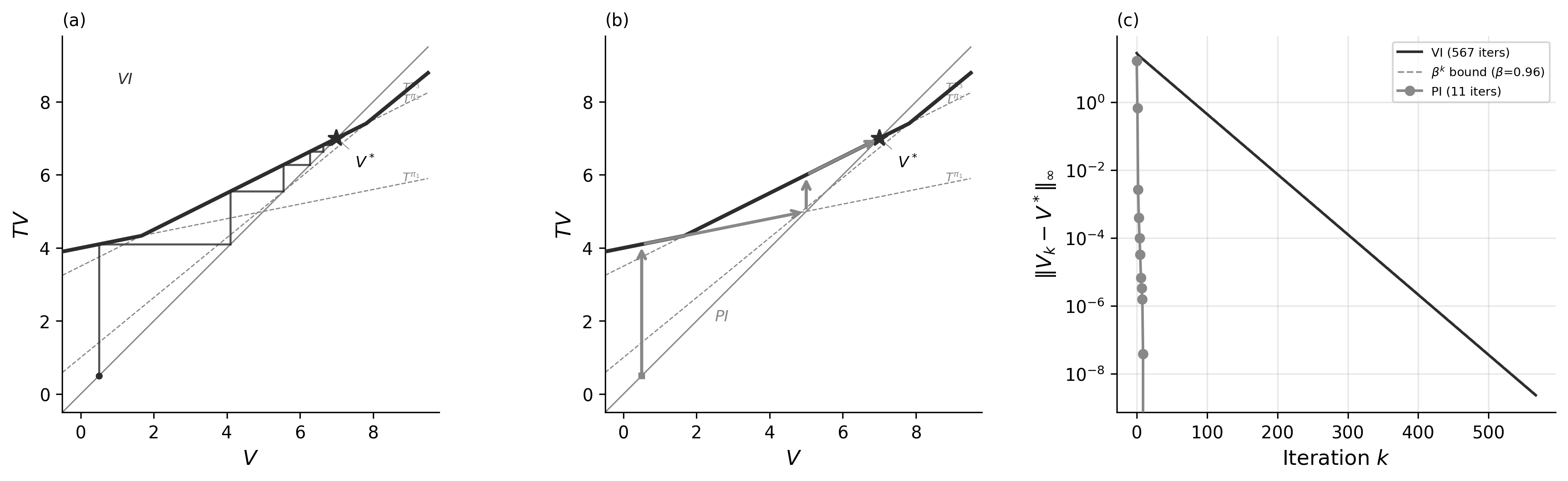
@blackwell1965 established the measure-theoretic foundations for discounted dynamic programming with general state and action spaces. He proved that the Bellman operator $T$ defined by $Tu(s) = \sup_a [r(s,a) + \gamma \int u(s') P(ds'|s,a)]$ is a contraction with modulus $\gamma$: $\|Tu - Tv\|_\infty \leq \gamma \|u - v\|_\infty$. Banach's fixed-point theorem then guarantees a unique bounded solution $V^*$ to the Bellman equation, with $\|V_k - V^*\|_\infty \leq \gamma^k \|V_0 - V^*\|_\infty$ under value iteration. The central result concerns stationary policies, which use the same decision rule $f: \mathcal{S} \to \mathcal{A}$ at every period regardless of history. Blackwell proved that if the action space is finite, there exists an optimal stationary policy. For countable action spaces, $\epsilon$-optimal stationary policies exist for every $\epsilon > 0$. These results justify the focus on memoryless policies, since optimal behavior depends only on the current state, not on the history of past states and actions. The Bellman equation, Howard's policy iteration, and Blackwell's existence theorems constitute the planning framework. Given complete knowledge of $P$ and $r$, these methods compute optimal policies exactly. The challenge of learning without such knowledge is the central problem of reinforcement learning.[^21]
# Reinforcement Learning Algorithms {#section:rl_algorithms}
## The Classical Synthesis {#sec:classical_synthesis}
### Monte Carlo Estimation
When $P(s'|s,a)$ and $r(s,a)$ are unknown, the obvious approach is to use Monte Carlo (MC) to approximate them. These methods estimate value functions from sampled *episodes* $(s_0, a_0, r_1, s_1, a_1, r_2, \ldots, s_T)$. The realized *return* from state $s_t$ is $$G_t = \sum_{k=0}^{T-t-1} \gamma^k r_{t+k+1}$$ First-visit MC prediction averages $G_t$ over episodes for each state $s$, counting only its first occurrence per episode. Each first-visit return is an independent draw from the return distribution, so the sample mean converges almost surely to $V^\pi(s)$ by the strong law of large numbers [@sutton2018]. An incremental update is, $$V(s) \leftarrow V(s) + \alpha[G_t - V(s)]$$
For MC control, we can estimate action-values $Q(s,a)$ by averaging first-visit returns from each state-action pair, then improve the policy greedily: $\pi(s) = \mathop{\it argmax}_a Q(s,a)$. Under exploring starts (every $(s,a)$ pair begins an episode infinitely often), this alternation converges to $Q^*$. [^22]
### Sutton (1988)
Monte Carlo has two limitations. The agent must wait for episode termination to compute $G_t$, ruling out continuing tasks. And $G_t$ is unbiased ($\mathbb{E}[G_t \mid S_t = s] = V^\pi(s)$) but high-variance, because it sums random rewards over the entire *trajectory*.
@sutton1988 proposed temporal difference (TD) learning to fix both problems. TD(0) replaces the full return $G_t$ with a one-step target: $$V(s_t) \leftarrow V(s_t) + \alpha \left[ r_{t+1} + \gamma V(s_{t+1}) - V(s_t) \right]$$ The target $r_{t+1} + \gamma V(s_{t+1})$ depends on one random reward and one random transition, so its variance is low. The cost is bias. The bootstrap target $V(s_{t+1})$ is the agent's current estimate, not the true value. This is "*bootstrapping*".[^23] As $V$ improves, the bias shrinks; the low variance persists regardless. Sutton demonstrated this tradeoff on a five-state random walk where TD(0) converged faster than Monte Carlo with less data.
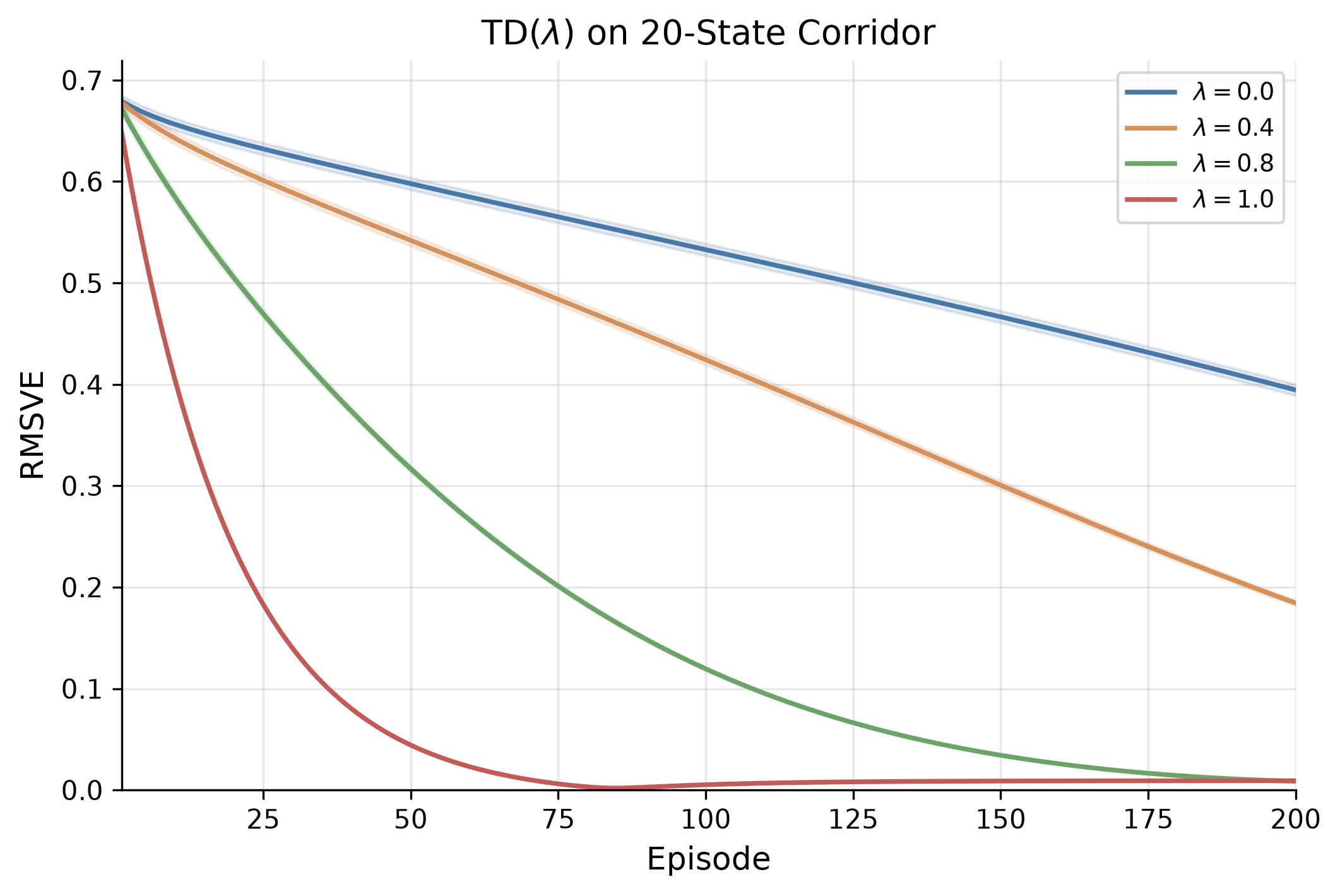
The general TD($\lambda$) update interpolates between these extremes through an eligibility trace.[^24] $$V(s_t) \leftarrow V(s_t) + \alpha \, \delta_t \, e_t(s)$$ where $\delta_t = r_{t+1} + \gamma V(s_{t+1}) - V(s_t)$ is the TD error and $e_t(s) = \gamma \lambda \, e_{t-1}(s) + \mathbbm{1}\{s = s_t\}$ is the eligibility trace for state $s$. Setting $\lambda = 0$ yields TD(0); setting $\lambda = 1$ recovers Monte Carlo returns. Intermediate $\lambda$ trades off variance against bias. [^25]
### Watkins (1989)
TD(0) learns value functions $V(s)$, but converting these to actions (the control problem) still requires knowing transition probabilities. Given $V(s')$ for all successor states, the agent needs to know which action leads to which successor.
@WatkinsDayan1992, formalizing Watkins's 1989 PhD thesis, provided the solution. Instead of learning $V(s')$ learn $Q(s,a)$ (the action value function or the "quality\" of actions function) directly, the expected return from taking action $a$ in state $s$ and then behaving optimally. The optimal policy is then $\pi^*(s) = \mathop{\it argmax}_a Q^*(s,a)$, requiring no model to act. The Bellman optimality equation provides the fixed-point condition: $$Q^*(s,a) = \mathbb{E}\left[r + \gamma \max_{a'} Q^*(s',a') \mid s, a\right]$$ Q-learning achieves this via the update $$Q(s_t, a_t) \leftarrow Q(s_t, a_t) + \alpha \left[ r_{t+1} + \gamma \max_{a'} Q(s_{t+1}, a') - Q(s_t, a_t) \right]$$ Q-learning converges to $Q^*$ under standard regularity conditions (Section [5.2](#sec:stochastic_approx){reference-type="ref" reference="sec:stochastic_approx"}). The maximization over $a'$ makes Q-learning *off-policy*:[^26] the update target uses the greedy action at the next state regardless of the action actually taken. Therefore the agent can follow an $\varepsilon$-greedy exploration strategy or even a fully random policy, while learning about the optimal policy directly.
### Williams (1992)
Value-based methods learn an action-value function and derive a policy from it. @williams1992 derived an alternative, policy gradients, that optimize the policy directly by gradient ascent on expected return $$\nabla_\theta J(\theta) = \mathbb{E}_{\pi_\theta} \left[ \sum_{t=0}^{T} \nabla_\theta \log \pi_\theta(a_t|s_t) \, G_t \right]$$ where $G_t = \sum_{k=0}^{T-t} \gamma^k r_{t+k+1}$ is the discounted return from time $t$. The log-derivative trick allows the gradient to be estimated from sampled trajectories without differentiating through the environment dynamics.
Consider a robot arm that must apply a continuous torque $a \in \mathbb{R}$ to reach a target angle. Q-learning requires computing $\max_a Q(s,a)$ at every update, which becomes a nested optimization problem [^27] when the action space is continuous. A policy gradient method sidesteps the issue. Parameterize the policy as a Gaussian $\pi_\theta(a|s) = \mathcal{N}(\mu_\theta(s),\, \sigma_\theta^2(s))$,[^28] sample an action, observe the return, and update $\theta$ by REINFORCE. Virtually all continuous-control results in reinforcement learning descend from the policy gradient framework for this reason.
### Tesauro (1994)
@tesauro1994's TD-Gammon demonstrated that temporal difference learning with neural network function approximation could achieve expert-level play in a domain with approximately $10^{20}$ legal positions[^29].
Backgammon was far beyond tabular methods, yet TD-Gammon trained a feedforward neural network to estimate the probability of winning from any board position. A hidden layer[^30] of 80 sigmoid units fed a single sigmoid output. $$\hat{V}(s) = \sigma\!\bigl(\mathbf{w}^\top \sigma(W\mathbf{x}(s) + \mathbf{b}) + c\bigr)$$ where $\sigma$ is the logistic sigmoid, $W$ is the input-to-hidden weight matrix, and $\mathbf{w}$ is the hidden-to-output weight vector. The network was trained by self-play using TD($\lambda$) with $\lambda = 0.7$. After each move from position $s_t$ to $s_{t+1}$, the weights $\boldsymbol{\theta}$[^31] were updated by $$\boldsymbol{\theta} \leftarrow \boldsymbol{\theta} + \alpha \bigl[\hat{V}(s_{t+1}) - \hat{V}(s_t)\bigr] \, \mathbf{e}_t$$ where $\alpha$[^32] is the step size, and the eligibility trace $\mathbf{e}_t = \sum_{k=1}^{t} \lambda^{t-k} \nabla_{\boldsymbol{\theta}} \hat{V}(s_k)$ accumulates exponentially decayed gradients of past predictions.[^33] At game's end, $\hat{V}(s_{t+1})$ is replaced by the outcome $z \in \{0, 1\}$.
A single neural network $\hat{V}$ serves as the evaluation function for both players. At each turn, the current player selects the legal move maximizing $\hat{V}(s')$ from its own perspective. As the network improves, it generates stronger play on both sides, producing harder training games that drive further improvement. The dice rolls ensure diverse board positions without requiring an explicit exploration mechanism.[^34]
### SARSA (1994)
Q-learning learns the optimal action-value function regardless of the policy generating experience. This off-policy property is useful but introduces complications when combined with function approximation. @rummery1994 introduced SARSA as an *on-policy*[^35] alternative that learns the value of the policy actually being followed. The name derives from the quintuple $(s_t, a_t, r_{t+1}, s_{t+1}, a_{t+1})$ used in each update: $$Q(s_t, a_t) \leftarrow Q(s_t, a_t) + \alpha \left[ r_{t+1} + \gamma Q(s_{t+1}, a_{t+1}) - Q(s_t, a_t) \right]$$ The key difference from Q-learning is that SARSA bootstraps from the action $a_{t+1}$ actually taken at the next state, rather than the greedy action $\mathop{\it argmax}_{a'} Q(s_{t+1}, a')$. This makes the algorithm on-policy, since the target depends on the behavior policy generating the data.
If the agent follows an $\varepsilon$-greedy policy, SARSA converges to $Q^{\varepsilon\text{-greedy}}$, not $Q^*$[^36] policies and standard step-size conditions (Section [5.2](#sec:stochastic_approx){reference-type="ref" reference="sec:stochastic_approx"}). This distinction matters when exploration is costly. Consider the cliff-walking problem, where an agent must traverse a gridworld with a cliff along one edge. The optimal path runs along the cliff edge (shortest route), but the $\varepsilon$-greedy policy occasionally falls off. Q-learning learns the optimal path because it evaluates the greedy policy; the agent falls off during learning but the Q-values reflect the optimal route. SARSA learns a safer path further from the cliff because it evaluates the actual exploratory policy; it accounts for the fact that exploration sometimes leads to catastrophic states.
### Baird (1995)
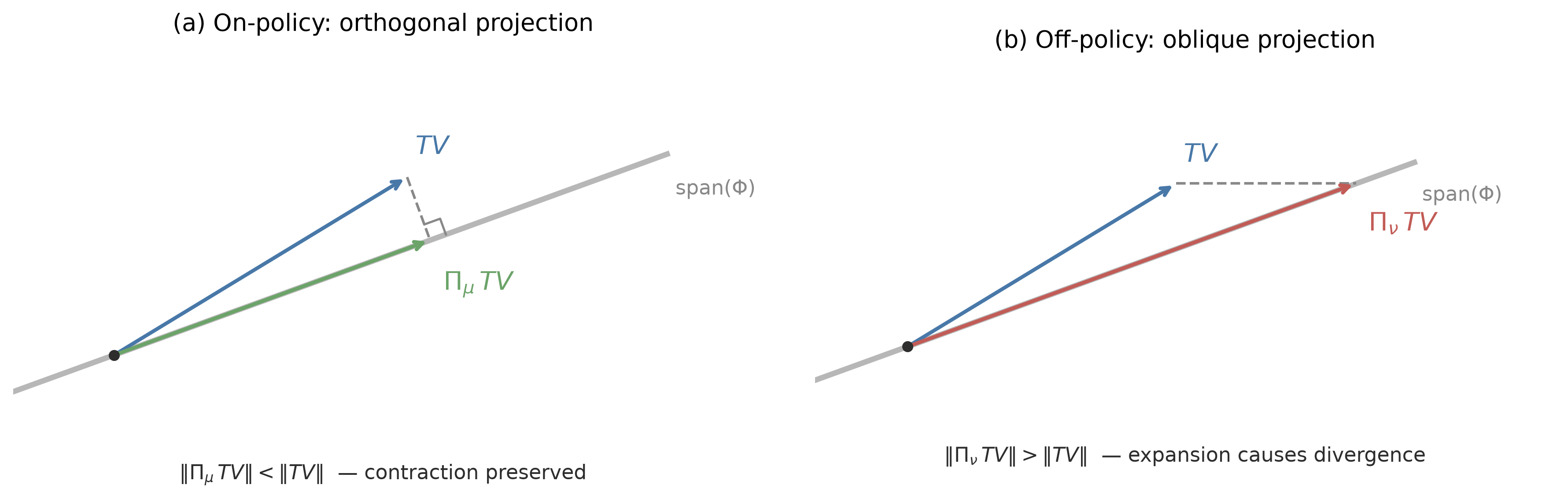
@Baird1995 constructed a six-state star MDP demonstrating divergence of Q-learning with linear function approximation. The MDP has five outer states that all transition to a single inner state under the target policy. The off-policy behavior samples states uniformly. With linear function approximation, the weights grow without bound under repeated Q-learning updates. The source of instability is the interaction of three components, namely bootstrapping (updating from estimated values rather than observed returns), off-policy learning (training on data from a different policy than the target), and function approximation (representing the value function with a parameterized model). @sutton2018 later named this the deadly triad. Any two components can be combined safely; all three together permit divergence. The mechanism underlying this instability is analyzed in Section [5.3](#sec:deadly_triad){reference-type="ref" reference="sec:deadly_triad"}.
This result explains the asymmetry between Tesauro's success and Baird's failure. TD-Gammon used bootstrapping and function approximation but was on-policy, with training data coming from the same self-play policy whose value was being estimated. Baird's counterexample used all three components and diverged. Baird also proposed a constructive solution, namely residual gradient algorithms that perform gradient descent on the mean-squared Bellman residual, guaranteeing convergence at the cost of a different fixed point.
### Actor-Critic Methods (2000)
The idea of maintaining both a policy (*actor*) and a value function (*critic*) dates to @barto1983neuronlike, who used a two-component system to solve the pole-balancing task. Actor-critic methods address the high variance of REINFORCE by replacing Monte Carlo returns with bootstrapped TD targets as the learning signal. The critic learns a value function $V(s)$ by TD updates. $$V(s_t) \leftarrow V(s_t) + \alpha_c \, \delta_t, \quad \delta_t = r_{t+1} + \gamma V(s_{t+1}) - V(s_t)$$ The actor updates the policy using the TD error as a sample of the advantage. $$\theta \leftarrow \theta + \alpha_a \nabla_\theta \log \pi_\theta(a_t|s_t) \, \delta_t$$ The TD error $\delta_t$ estimates $A^\pi(s_t, a_t) = Q^\pi(s_t, a_t) - V^\pi(s_t)$, the advantage of action $a_t$ over the average action.[^37] Positive advantages indicate the action was better than expected; negative advantages indicate it was worse.
@konda2000 provided the first convergence proof for actor-critic algorithms with function approximation, showing convergence to a stationary point under two-timescale learning rates ($\alpha_c \gg \alpha_a$) and a compatibility condition on the critic architecture (Section [5.5](#sec:actor_critic){reference-type="ref" reference="sec:actor_critic"}).
### Natural Policy Gradient (2001)
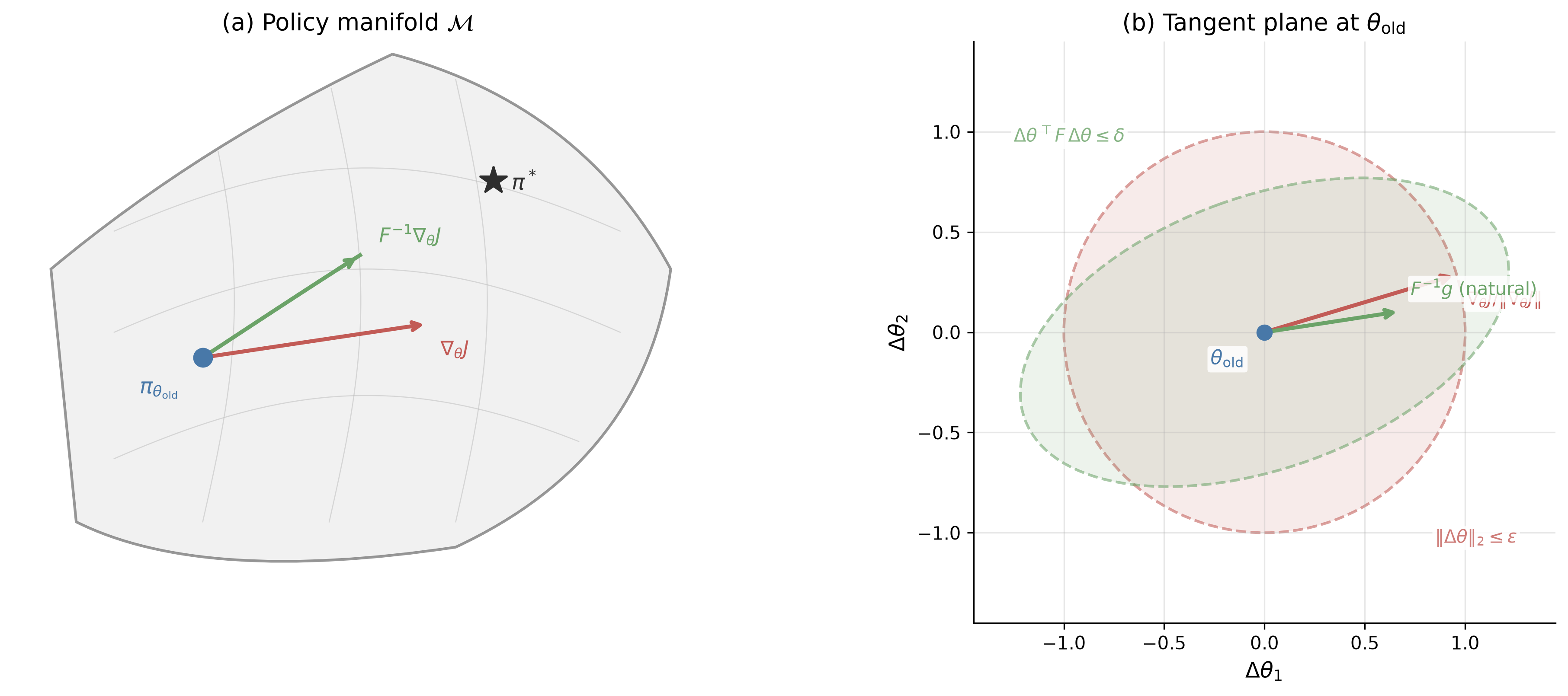
Standard gradient descent treats all parameter directions equally, but policy parameters define probability distributions whose natural geometry is not Euclidean. @Kakade2001 introduced the natural policy gradient, which measures progress in distribution space rather than parameter space. The update uses the Fisher information matrix $F(\theta)$: $$F(\theta) = \mathbb{E}_{s \sim d^\pi, a \sim \pi_\theta} \left[ \nabla_\theta \log \pi_\theta(a|s) \nabla_\theta \log \pi_\theta(a|s)^\top \right]$$ The natural gradient is $$\tilde{\nabla}_\theta J(\theta) = F(\theta)^{-1} \nabla_\theta J(\theta)$$ This direction is invariant to reparameterization of the policy. In the tabular softmax[^38] case, a single natural gradient step with unit step size recovers one step of exact policy iteration (Section [5.4](#sec:policy_gradient){reference-type="ref" reference="sec:policy_gradient"}).
The computational bottleneck is inverting $F(\theta) \in \mathbb{R}^{d \times d}$. Practical implementations use conjugate gradient methods to solve $F(\theta) x = \nabla_\theta J(\theta)$ without forming $F$ explicitly. This approach was later scaled to deep neural networks by TRPO and PPO.
### Fitted Value Iteration and Fitted Q-Iteration (2005) {#sec:fvi_fqi_algorithms}
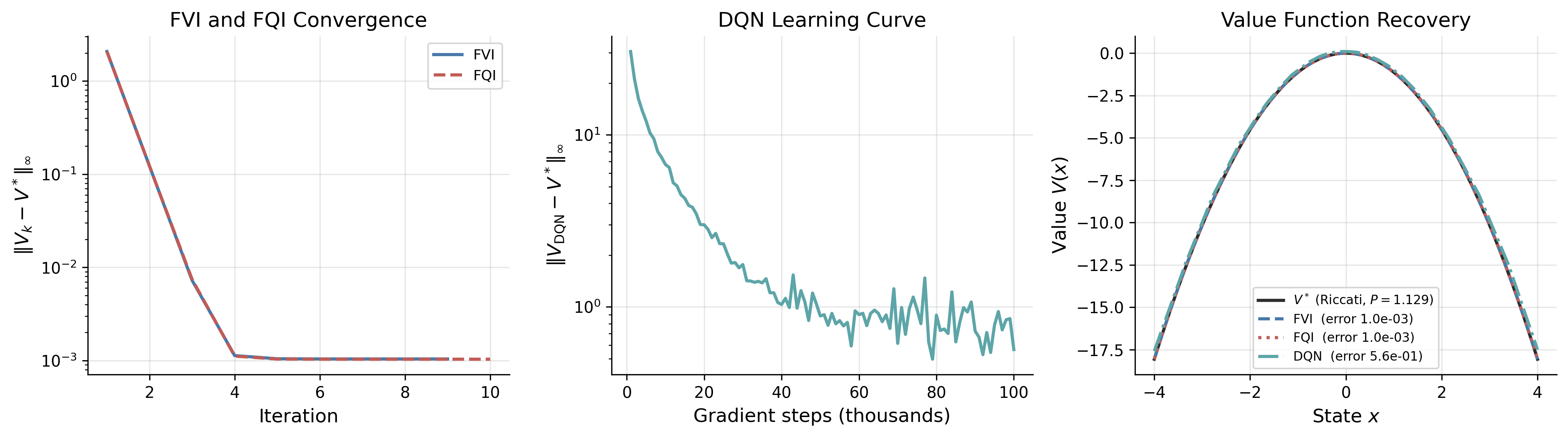
Tabular Q-learning maintains a separate entry for every state-action pair. When $|\mathcal{S}|$ is large or the state space is continuous, as in most applied problems, this is infeasible. *Fitted Q-Iteration* (FQI) [@Ernst2005] replaces the tabular update with a supervised regression step: given a batch of transitions, fit a function approximator to the Bellman targets.
Let $\mathcal{F}$ be a function class mapping $\mathcal{S} \times \mathcal{A} \to \mathbb{R}$.[]{#def:fqi label="def:fqi"} Initialize $Q_0 \equiv 0$. At each iteration $k = 0, 1, \ldots, K-1$: (i) draw $N$ transitions $(s_i, a_i, r_i, s_i')$ from a generative model; (ii) construct regression targets $y_i^{(k)} = r_i + \gamma \max_{a'} Q_k(s_i', a')$; (iii) set $Q_{k+1} \leftarrow \arg\min_{f \in \mathcal{F}} \frac{1}{N} \sum_{i=1}^N \bigl( f(s_i, a_i) - y_i^{(k)} \bigr)^2$. The output is the greedy policy $\pi_K(s) = \arg\max_a Q_K(s,a)$.
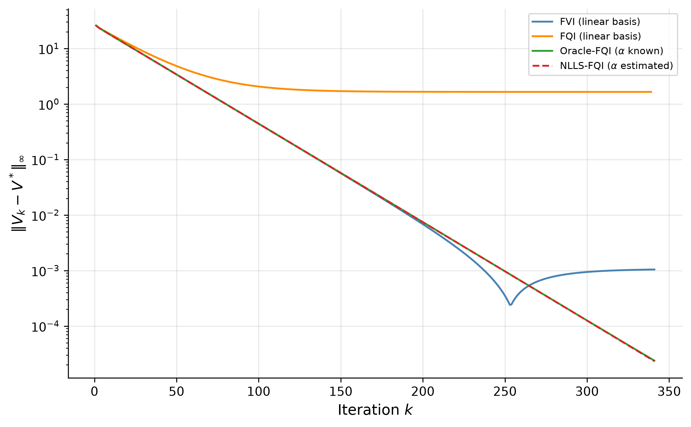
The regression step replaces the exact Bellman application with a projection onto $\mathcal{F}$: $Q_{k+1} = \Pi_{\mathcal{F}} \mathcal{T} Q_k$, where $\mathcal{T}$ is the Bellman optimality operator and $\Pi_{\mathcal{F}}$ is the $L^2$-projection under the sample distribution. Fitted Value Iteration (FVI) [@MunosSzepesvari2008] applies the same idea to the value function directly: $V_{k+1} = \Pi_{\mathcal{F}} \mathcal{T}^* V_k$, where $(\mathcal{T}^* V)(s) = \max_a \{ r(s,a) + \gamma \sum_{s'} P(s'|s,a) V(s') \}$.
With feature matrix $\Phi \in \mathbb{R}^{|\mathcal{S}| \times d}$ (rows $\phi(s)^\top$) and per-action weight vectors $\theta_a \in \mathbb{R}^d$, each FQI regression step for action $a$ reduces to the normal equations: $$\theta_a^{(k+1)} = \bigl(\Phi^\top \Phi\bigr)^{-1} \Phi^\top y_a^{(k)},
\label{eq:fqi_normal}$$ where $y_a^{(k)}(s) = r(s,a) + \gamma \sum_{s'} P(s'|s,a) \max_{a'} \phi(s')^\top \theta_{a'}^{(k)}$. Computation is $O(d^2 |\mathcal{S}| + d^3)$ per action per iteration. The FVI update takes the same form with a single weight vector $\theta_V$: $$\theta_V^{(k+1)} = \bigl(\Phi^\top \Phi\bigr)^{-1} \Phi^\top V_{\mathrm{target}}^{(k)},
\label{eq:fvi_normal}$$ where $V_{\mathrm{target}}^{(k)}(s) = \max_a \bigl\{ r(s,a) + \gamma \sum_{s'} P(s'|s,a) \phi(s')^\top \theta_V^{(k)} \bigr\}$. The finite-sample error theory for these methods is developed in Section [5.2.5](#sec:fvi_fqi_theory){reference-type="ref" reference="sec:fvi_fqi_theory"}.
## The Deep Learning Era
### Deep Q-Networks (2015)
@mnih2015 trained a single convolutional neural network[^39] to play 49 Atari 2600 games directly from pixel inputs ($210 \times 160 \times 3$) and a scalar score, using no game-specific features.
The architecture processed four consecutive frames through three convolutional layers and a fully connected layer.[^40] The network $Q(s, a; \theta)$ was trained to minimize the squared temporal difference error $$L(\theta) = \mathbb{E}_{(s,a,r,s') \sim \mathcal{D}} \left[ \left( r + \gamma \max_{a'} Q(s', a'; \theta^-) - Q(s, a; \theta) \right)^2 \right]$$
Two innovations stabilized learning. *Experience replay* [@Lin1992] stored transitions $(s, a, r, s')$ in a buffer $\mathcal{D}$ and sampled uniformly for training, breaking the temporal correlation between consecutive updates. A *target network* used a frozen copy of parameters $\theta^-$, updated periodically,[^41] so the regression target does not shift with each gradient step.
DQN exceeded human-level performance on 29 of 49 games using a single architecture and hyperparameters.[^42] Games requiring long-horizon planning or sparse rewards, such as Montezuma's Revenge, remained difficult.
### TRPO and PPO (2015, 2017)
Policy gradient methods suffer from a practical instability: a single large gradient step can move the policy into a region where performance collapses and recovery is slow.
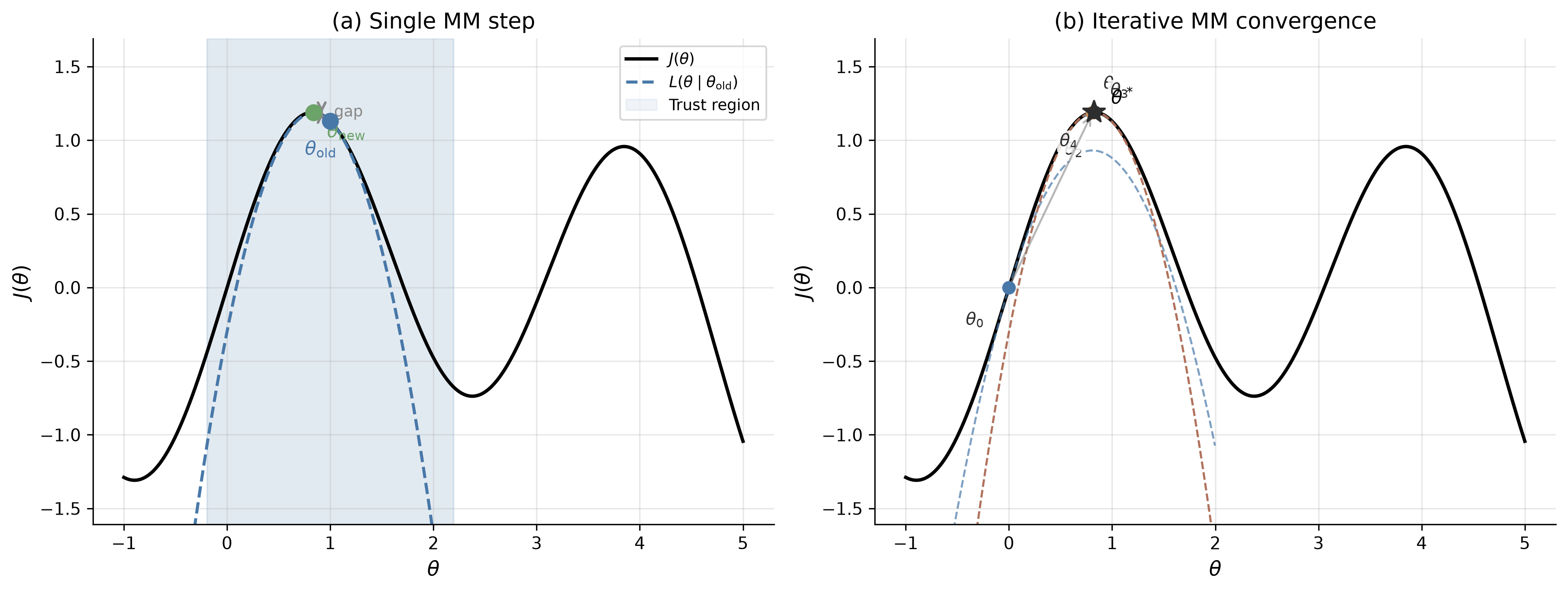
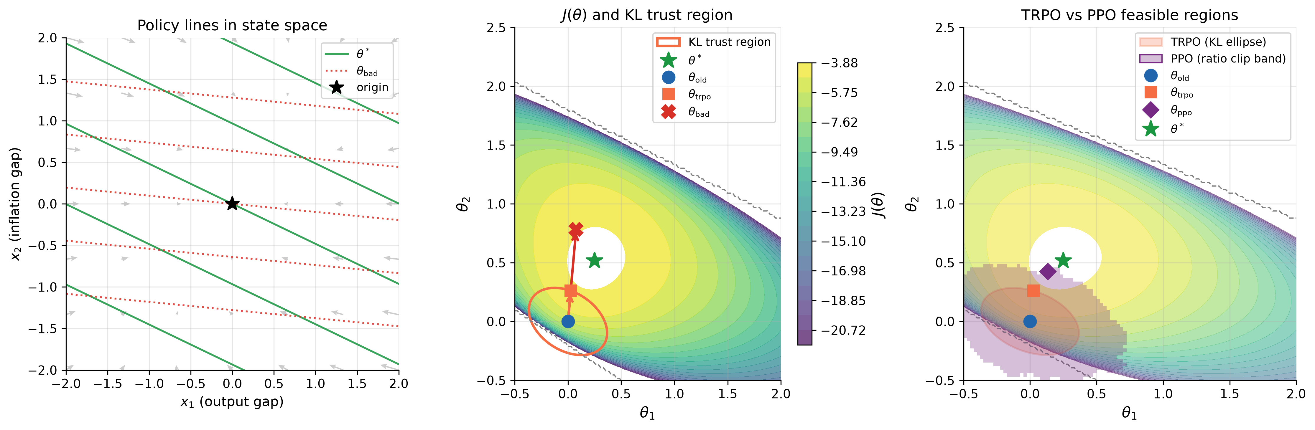
@Schulman2015 addressed this with Trust Region Policy Optimization (TRPO). TRPO solves the constrained optimization problem $$\max_\theta \; L_{\theta_{\text{old}}}(\theta) \quad \text{subject to} \quad \bar{D}_{\mathrm{KL}}(\theta_{\text{old}}, \theta) \leq \delta$$ where $L$ is a surrogate objective based on the advantage function $A^\pi(s,a) = Q^\pi(s,a) - V^\pi(s)$.[^43]
@Schulman2017 proposed Proximal Policy Optimization (PPO) as a simpler alternative. PPO replaces the KL constraint with a clipped surrogate objective: $$L^{\text{CLIP}}(\theta) = \mathbb{E}_t \left[ \min\!\left( r_t(\theta) \hat{A}_t, \; \text{clip}(r_t(\theta), 1-\varepsilon, 1+\varepsilon) \hat{A}_t \right) \right]$$ where $r_t(\theta) = \pi_\theta(a_t|s_t) / \pi_{\theta_{\text{old}}}(a_t|s_t)$ is the probability ratio. The clipping removes the incentive for $r_t(\theta)$ to move outside the interval $[1-\varepsilon, 1+\varepsilon]$, penalizing large policy updates without explicitly computing a divergence measure.
PPO outperformed A2C, TRPO, and the cross-entropy method on continuous control benchmarks and achieved the highest average reward on 30 of 49 Atari games among the methods tested. PPO became the default policy optimization algorithm for large-scale RL applications, demonstrating that constraining the magnitude of policy updates is essential for stable optimization.
### Soft Actor-Critic (2018)
@Haarnoja2018 introduced Soft Actor-Critic (SAC), which adds entropy regularization to the actor-critic framework. The agent maximizes expected return plus an entropy bonus: $$J(\theta) = \mathbb{E}_{\pi_\theta}\left[\sum_{t=0}^\infty \gamma^t \left(r_t + \tau \mathcal{H}(\pi_\theta(\cdot|s_t))\right)\right]$$ where $\mathcal{H}(\pi) = -\sum_a \pi(a) \log \pi(a)$ is the entropy and $\tau > 0$ is a temperature parameter. The entropy bonus encourages exploration by penalizing deterministic policies. The optimal policy under this objective is softmax in the Q-values: $\pi^*(a|s) \propto \exp(Q^*(s,a)/\tau)$, connecting to discrete choice models in econometrics.
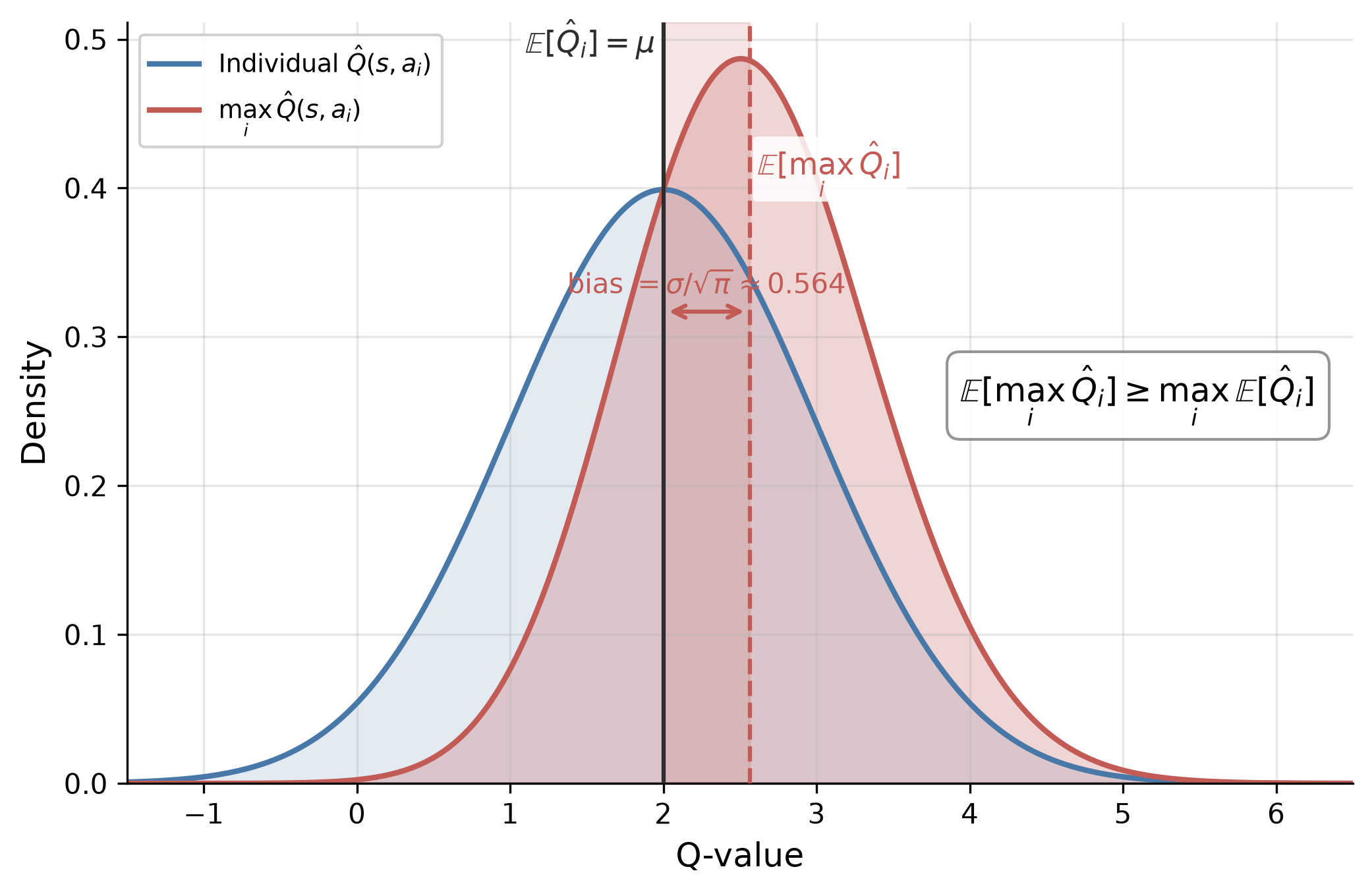
SAC maintains two Q-networks (to reduce overestimation bias) and a policy network. The soft Bellman operator for the critic is: $$(T^\pi Q)(s,a) = r(s,a) + \gamma \mathbb{E}_{s'}\left[ V(s') \right], \quad V(s) = \mathbb{E}_{a \sim \pi}[Q(s,a) - \tau \log \pi(a|s)]$$ SAC is off-policy (using experience replay), handles continuous actions naturally, and achieves state-of-the-art sample efficiency on continuous control benchmarks. The entropy regularization provides automatic exploration without $\varepsilon$-greedy schedules.
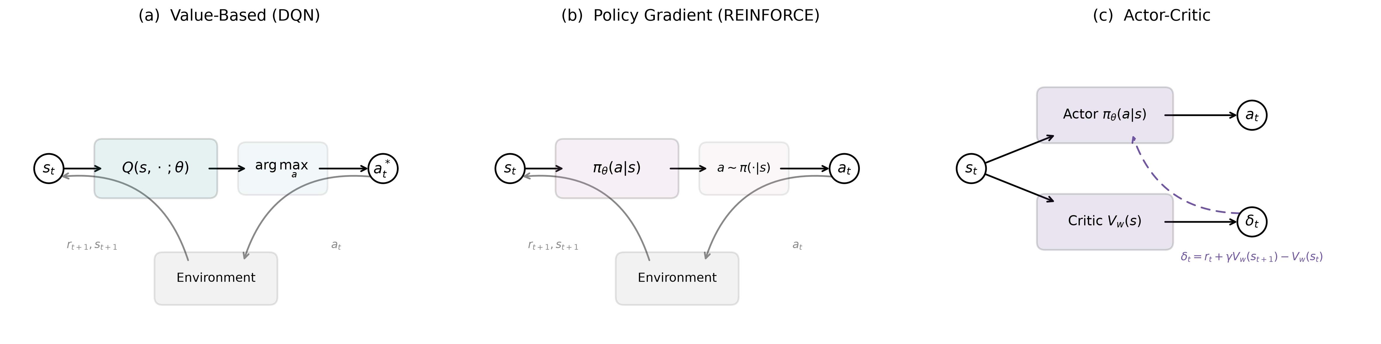
<span id="fig:algorithm_architectures"></span>
```{python}
#| label: fig-algorithm-architectures
#| fig-cap: "Architecture comparison of the three fundamental algorithm families. (a) DQN maps states to Q-values for all actions, selecting the argmax. (b) REINFORCE maps states to a probability distribution over actions, then samples. (c) Actor-Critic maintains separate policy and value networks; the critic's TD error $\\delta_t$ provides a low-variance learning signal to the actor."
script = "ch02_rl_algorithms/sims/algorithm_architectures.py"
output = "ch02_rl_algorithms/sims/algorithm_architectures.png"
artifacts = run_artifact(
    script=script,
    outputs=[output],
    mode="run",
    timeout=1800,
    reason="",
)
display_image(artifacts[output])
```
### Control as Probabilistic Inference {#sec:control_inference}
The *control-as-inference* framework [@Todorov2006; @Kappen2011; @Ziebart2010; @Levine2018] recasts the preceding algorithms as instances of probabilistic inference (computation, not statistical inference) in a single graphical model.[^44] The payoff is that every advance in approximate inference (variational methods, message passing, amortized inference) becomes a candidate RL algorithm, and the forward problem (finding the optimal policy given rewards) and the inverse problem (recovering rewards from observed behavior) become two queries in the same model. The construction introduces a binary "optimality" variable $\mathcal{O}_t \in \{0,1\}$ at each time step, appended to the standard state-action-dynamics chain (Figure [2](#fig:control_inference_dag){reference-type="ref" reference="fig:control_inference_dag"}). The distribution over this variable is defined as $$P(\mathcal{O}_t = 1 \mid s_t, a_t) = \exp(r(s_t, a_t)/\tau)
\label{eq:optimality_variable}$$ where $\tau > 0$ is a temperature parameter and rewards satisfy $r \leq 0$.[^45] This is a modeling assumption, not a derivation from first principles; the exponential form is chosen so the resulting posterior matches entropy-regularized RL.
<figure id="fig:control_inference_dag">
<figcaption>The control-as-inference graphical model. States <span class="math inline"><em>s</em><sub><em>t</em></sub></span> and actions <span class="math inline"><em>a</em><sub><em>t</em></sub></span> jointly determine the next state <span class="math inline"><em>s</em><sub><em>t</em> + 1</sub></span> (dynamics) and the optimality variable <span class="math inline">𝒪<sub><em>t</em></sub></span> (reward signal). Optimality nodes <span class="math inline">𝒪<sub><em>t</em></sub></span> are observed as <span class="math inline">𝒪<sub><em>t</em></sub> = 1</span>; the posterior over actions <span class="math inline"><em>P</em>(<em>a</em><sub><em>t</em></sub> ∣ <em>s</em><sub><em>t</em></sub>, 𝒪<sub><em>t</em> : <em>T</em></sub> = 1)</span> yields the optimal policy.</figcaption>
</figure>
The RL problem becomes a probabilistic inference query. Given that all future time steps are optimal ($\mathcal{O}_{t:T} = 1$), what is $P(a_t \mid s_t, \mathcal{O}_{t:T} = 1)$? Define backward messages $\beta_t(s, a) = P(\mathcal{O}_{t:T} = 1 \mid s_t = s,\, a_t = a)$, the probability that everything from $t$ onward is optimal given the agent is in state $s$ taking action $a$. These are computed by backward recursion: $$\begin{aligned}
\beta_T(s, a) &= \exp(r(s, a)/\tau) \label{eq:beta_base} \\
\beta_t(s, a) &= \exp(r(s, a)/\tau) \sum_{s'} P(s'|s,a) \, \beta_{t+1}(s') \quad (t < T) \label{eq:beta_recursion}
\end{aligned}$$ where $\beta_{t+1}(s') \propto \sum_{a'} \beta_{t+1}(s', a')$ marginalizes over future actions under a uniform prior. By Bayes' rule, the posterior over actions is $P(a_t \mid s_t, \mathcal{O}_{t:T} = 1) = \beta_t(s_t, a_t) \,/\, \sum_{a'} \beta_t(s_t, a')$. Defining $Q(s,a) = \tau \log \beta_t(s,a)$, so that backward messages in log-space correspond to soft value functions, and $V(s) = \tau \log \sum_a \exp(Q(s,a)/\tau)$[^46], the posterior becomes $\pi(a \mid s) = \exp\bigl((Q(s,a) - V(s))/\tau\bigr)$, the softmax over Q-values.
Exact inference in this graphical model under stochastic dynamics produces risk-seeking policies. The backup becomes $Q(s,a) = r(s,a) + \tau \log \mathbb{E}_{s'}[\exp(V(s')/\tau)]$, which overweights unlikely favorable transitions because the agent implicitly assumes it can influence the dynamics.[^47] The framework corrects this by applying structured variational inference, restricting the variational family to distributions that match the true dynamics $P(s'|s,a)$. This yields the soft Bellman equations $$\begin{aligned}
Q(s,a) &= r(s,a) + \gamma \, \mathbb{E}_{s' \sim P}[V(s')] \label{eq:soft_bellman_q} \\
V(s) &= \tau \log \sum_{a \in \mathcal{A}} \exp\!\left(\frac{Q(s,a)}{\tau}\right) \label{eq:soft_bellman_v}
\end{aligned}$$ with the optimal policy given by $\pi(a \mid s) = \exp\bigl((Q(s,a) - V(s))/\tau\bigr)$. The operator $\mathcal{T}^{\mathrm{soft}}$ defined by Equations [\[eq:soft_bellman_q\]](#eq:soft_bellman_q){reference-type="eqref" reference="eq:soft_bellman_q"}--[\[eq:soft_bellman_v\]](#eq:soft_bellman_v){reference-type="eqref" reference="eq:soft_bellman_v"} is a $\gamma$-contraction in $\|\cdot\|_\infty$, with the same convergence rate as the standard Bellman operator.[^48] As $\tau \to 0$, the log-sum-exp converges to the hard maximum and the soft Bellman equations reduce to the standard Bellman optimality equations. The value function in Equation [\[eq:soft_bellman_v\]](#eq:soft_bellman_v){reference-type="eqref" reference="eq:soft_bellman_v"} is identical to McFadden's social surplus function from discrete choice theory [@McFadden1978], completing the connection noted in the preceding subsection.
Classical RL already employs exploration strategies ($\varepsilon$-greedy, UCB), but these are designed separately from the optimization objective. In the probabilistic framework, the objective itself maximizes expected reward and policy entropy simultaneously.[^49] The Q-function, the value function, and the exploration behavior are all derived from a single objective. Different approximation strategies applied to this single model recover familiar algorithms. When the backward messages in Equations [\[eq:beta_base\]](#eq:beta_base){reference-type="eqref" reference="eq:beta_base"}--[\[eq:beta_recursion\]](#eq:beta_recursion){reference-type="eqref" reference="eq:beta_recursion"} are computed exactly in the tabular setting, the result is soft value iteration. Estimating the ELBO gradient via the likelihood ratio trick yields max-ent policy gradients, identical to REINFORCE with $-\tau \log \pi(a_t|s_t)$ added to the reward at each step. Fitting parameterized $Q_\phi$ and $V_\psi$ networks to approximate the backward messages gives Soft Actor-Critic [@Haarnoja2018]. Fitting $Q_\phi$ alone and extracting the policy implicitly via the softmax gives soft Q-learning [@Haarnoja2017]. Trust-region methods such as TRPO and PPO do not optimize the max-ent objective, but each policy update step solves a max-ent subproblem with the old policy as prior, so the per-step structure mirrors the framework even though the global target remains standard reward maximization [@Schulman2015; @Schulman2017]. Hard-max algorithms (Q-learning, DQN, standard policy gradient) are not direct instances of the framework; they are recovered in the zero-temperature limit $\tau \to 0$, where the softmax collapses to the argmax. Reading the graphical model in the reverse direction, treating the reward as the unknown and observed behavior as evidence of optimality, yields maximum entropy inverse reinforcement learning [@Ziebart2008], connecting to the structural estimation methods discussed in Section [8](#section:rl_econ_models){reference-type="ref" reference="section:rl_econ_models"}.
The framework has practical limitations. The converged fixed point is $Q^*_{\mathrm{soft}}$, not $Q^*$; at any $\tau > 0$, the policy is suboptimal for the original reward-maximization objective. The entropy bonus produces undirected exploration, spreading probability mass rather than targeting uncertain states. In safety-critical environments, the objective assigns nonzero probability to catastrophic actions. The practical benefits of the probabilistic perspective, including robustness to model perturbations and smooth optimization landscapes, are most apparent in continuous-control and robotics settings. In perfectly simulated environments with exact rewards (Atari, Go), the hard-max algorithms that dominate those domains do not require this probabilistic formulation, as the following subsection illustrates.
### AlphaGo Zero (2017) {#subsubsec:alphago_zero}
The game of Go has approximately $10^{170}$ legal positions and a branching factor of roughly 250, far beyond the reach of brute-force search. Hand-crafted evaluation functions, which had succeeded in chess, failed here because positional concepts like influence, territory, and group viability are holistic and contextual. Monte Carlo tree search (MCTS) had achieved amateur-level play by using random simulations to estimate position values, but progress had stalled below professional strength. @Silver2016 broke through by combining supervised learning from 30 million human expert positions, reinforcement learning via self-play, and MCTS with learned value and policy networks; the resulting system defeated Lee Sedol four games to one in March 2016. A year later, @Silver2017 showed that none of the human data was necessary.
AlphaGo Zero uses a single convolutional neural network $f_\theta(s) = (\mathbf{p}, v)$ that takes a board position $s$ and outputs both a policy vector $\mathbf{p}$ over legal moves and a scalar value $v$ estimating the probability of winning. The input representation consists of 17 binary planes on the $19 \times 19$ board encoding the raw game state without hand-crafted features.[^50] The architecture uses residual blocks,[^51] which allow training of very deep networks.
During play, each move is selected by running MCTS, which conducts 1,600 simulated games from the current position to estimate move quality. Each simulation proceeds in four phases, illustrated in Figure [3](#fig:mcts_phases){reference-type="ref" reference="fig:mcts_phases"}. In the selection phase, the algorithm starts from the current position and traverses the partially built search tree by choosing at each node the action that maximizes $Q(s,a) + c_{\text{puct}} \cdot P(s,a) \cdot \sqrt{\sum_b N(s,b)} \,/\, (1 + N(s,a))$, where $Q(s,a)$ is the current average value of action $a$, $P(s,a)$ is the prior probability from the neural network, and $N(s,a)$ is the visit count.[^52] In the expansion and evaluation phase, when the traversal reaches a position not yet in the tree, the neural network evaluates it in a single forward pass, producing a policy vector $\mathbf{p}$ and a value estimate $v$; the policy initializes prior probabilities $P(s',a) = p_a$ for each child edge. In the backup phase, the value $v$ propagates back up the traversed path, incrementing each edge's visit count $N(s,a)$ and updating its mean value $Q(s,a)$. After all 1,600 simulations, the algorithm selects the move with the highest visit count at the root.
<figure id="fig:mcts_phases">
<figcaption>The four phases of a single MCTS simulation in AlphaGo Zero. (a) Selection traverses the tree from the root, choosing at each node the action maximizing a UCB-like score balancing exploitation (<span class="math inline"><em>Q</em></span>) and exploration (<span class="math inline"><em>P</em>/<em>N</em></span>). (b) Expansion adds a new leaf node when the traversal reaches an unexplored position. (c) The neural network <span class="math inline"><em>f</em><sub><em>θ</em></sub></span> evaluates the new position, producing move priors <span class="math inline"><strong>p</strong></span> and a value estimate <span class="math inline"><em>v</em></span>. (d) Backup propagates <span class="math inline"><em>v</em></span> along the traversed path, updating mean values <span class="math inline"><em>Q</em>(<em>s</em>, <em>a</em>)</span> and visit counts <span class="math inline"><em>N</em>(<em>s</em>, <em>a</em>)</span> at each edge.</figcaption>
</figure>
The training loop generates self-play games. At each board position $s_t$ during a game, the program runs MCTS to produce improved move probabilities $\boldsymbol{\pi}_t$, where $\pi_t(a) \propto N(s_t, a)^{1/\tau}$ and $\tau$ is a temperature parameter controlling exploration.[^53] A move $a_t$ is sampled from $\boldsymbol{\pi}_t$ and played. At game end, the outcome $z \in \{-1, +1\}$ is recorded. Each position becomes a training triple $(s_t, \boldsymbol{\pi}_t, z)$, and the network parameters are updated to minimize $$\ell(\theta) = (z - v)^2 - \boldsymbol{\pi}^\top \log \mathbf{p} + c \|\theta\|^2$$ where the first term is a value prediction loss, the second is a policy cross-entropy loss,[^54] and the third is $L_2$ regularization.[^55] The key mechanism is a virtuous cycle. MCTS serves as a policy improvement operator, since the search probabilities $\boldsymbol{\pi}$ are stronger than the raw network outputs $\mathbf{p}$. Training the network to match $\boldsymbol{\pi}$ distills the search improvements back into the network, and the improved network in turn produces better MCTS. After 72 hours of self-play on 4 TPUs, AlphaGo Zero surpassed all previous versions, including the one that defeated Lee Sedol, and discovered novel strategies not previously seen in human play.[^56]
Go was well-suited to this architecture. Its fixed $19 \times 19$ board maps naturally to convolutional networks, its perfect information and deterministic transitions make MCTS's tree structure exact, and the binary game outcome provides an unambiguous training signal. @Igami2020 interprets the architecture in econometric terms, where the policy network is a conditional choice probability (CCP) estimator, the value network is a conditional value function (CVF) estimator, and the system performs CCP estimation and forward simulation jointly, connecting to the approach of @HotzMiller1993 in dynamic discrete choice.
### Decision Transformers (2021) {#subsubsec:decision_transformers}
@Chen2021DT proposed replacing Bellman backups with autoregressive sequence modeling. The Decision Transformer conditions a causal GPT-style Transformer on trajectories $\tau = (\hat{R}_1, s_1, a_1, \hat{R}_2, s_2,
a_2, \ldots)$, where $\hat{R}_t$ is the *return-to-go* (desired future cumulative reward). At test time, conditioning on a high target return extracts a high-performing policy without any temporal-difference learning. @Janner2021TT extended this to the Trajectory Transformer, modeling entire trajectories as flat token sequences with continuous dimensions discretized into bins, enabling planning via beam search over trajectories.
The approach has fundamental limitations that Bellman-based methods do not share. @Brandfonbrener2022 proved that return-conditioned supervised learning (RCSL) recovers optimal policies only under assumptions strictly stronger than those needed for dynamic programming: near-deterministic dynamics, expert data coverage, and a unique mapping from returns to optimal actions. In stochastic environments, high returns may reflect environmental luck rather than good decisions, causing RCSL to imitate lucky-but-suboptimal trajectories. @Paster2022 demonstrated this concretely: in a simple gambling MDP, the Decision Transformer conditioned on high returns selects risky gambles over the optimal safe action, even with infinite data.[^57]
A second limitation is that RCSL cannot *stitch* suboptimal trajectory segments. If the dataset contains two trajectories that each visit a useful intermediate state but from different starting points, Bellman-based methods can compose the better segments by propagating values backward through the shared state. Sequence models, which predict forward autoregressively, cannot perform this backward composition.
# The Theory of Reinforcement Learning {#sec:planning_learning}
## The Geometry of Dynamic Programming {#sec:newton_connection}
Value iteration (VI) and policy iteration (PI) are the workhorses of dynamic programming. VI applies the Bellman operator repeatedly until convergence; PI alternates between *policy evaluation* (solving a linear system) and *policy improvement* (taking the greedy action). PI converges faster. Why? The answer reveals a connection between dynamic programming and numerical optimization. Policy iteration is Newton's method applied to the Bellman equation.
### Value Iteration as Picard Iteration
Consider the Bellman optimality operator $T$ acting on value functions. $$(TV)(s) = \max_{a \in \mathcal{A}} \left\{ r(s,a) + \gamma \sum_{s' \in \mathcal{S}} P(s'|s,a) V(s') \right\}.
\label{eq:bellman_operator}$$ This operator is nonlinear due to the $\max$. Value iteration applies $T$ repeatedly: $V_{k+1} = TV_k$. Since $T$ is a $\gamma$-contraction in the supremum norm [@denardo1967], Banach's fixed-point theorem guarantees $\|V_k - V^*\|_\infty \leq \gamma^k \|V_0 - V^*\|_\infty$.[^58] This is Picard iteration, with linear convergence at rate $\gamma$.[^59] The iteration count to reduce error by a factor of $\delta$ is $k = \log(\delta) / \log(1/\gamma)$ [@bertsekas1996].
### Policy Iteration as Newton's Method
Policy iteration takes a different approach. At the current value estimate $\tilde{V}$, define the greedy policy $\tilde{\pi}(s) = \mathop{\it argmax}_a \{ r(s,a) + \gamma \sum_{s'} P(s'|s,a) \tilde{V}(s') \}$. The *policy evaluation* step solves the linear fixed-point equation $V = T^{\tilde{\pi}} V$ exactly, where $T^{\tilde{\pi}}$ is the policy-specific Bellman operator $$(T^{\tilde{\pi}} V)(s) = r(s, \tilde{\pi}(s)) + \gamma \sum_{s'} P(s'|s,\tilde{\pi}(s)) V(s').$$
The geometric structure, formalized by @puterman1979, is as follows: the linear operator $T^{\tilde{\pi}}$ is a supporting hyperplane to the nonlinear operator $T$ at the current iterate.[^60] Specifically, the operators satisfy tangency: $T^{\tilde{\pi}} \tilde{V} = T\tilde{V}$, so the linearization agrees with the nonlinear operator at the current iterate. They also satisfy support: $T^{\tilde{\pi}} V \leq TV$ for all $V$, meaning the linear operator lies weakly below the nonlinear one everywhere, just as a tangent line lies below a convex function. Policy evaluation solves for the fixed point of this linearization exactly. This is precisely the structure of Newton's method; linearize the nonlinear equation at the current point, solve the linearized system, and iterate.[^61][^62]
::: {#thm:policy_improvement .theorem}
**Theorem 1** (Policy Improvement, @howard1960). *Let $\pi_k$ be the current policy with value $V^{\pi_k}$, and let $\pi_{k+1}$ be the greedy policy with respect to $V^{\pi_k}$: $$\pi_{k+1}(s) = \mathop{\it argmax}_{a \in \mathcal{A}} \left\{ r(s,a) + \gamma \sum_{s'} P(s'|s,a)\, V^{\pi_k}(s') \right\}.$$ Then $V^{\pi_{k+1}}(s) \geq V^{\pi_k}(s)$ for all $s \in \mathcal{S}$, with strict inequality at some state unless $\pi_k$ is already optimal.*
:::
The consequence is finite termination. Since there are at most $|\mathcal{A}|^{|\mathcal{S}|}$ deterministic policies and each PI step strictly improves the value function (Theorem [1](#thm:policy_improvement){reference-type="ref" reference="thm:policy_improvement"}), PI reaches the exact optimum in finitely many iterations. While VI requires $k = \log(100) / \log(1/\gamma)$ iterations to reduce error by a factor of 100 [@bertsekas1996], PI typically converges in 5--10 iterations regardless of $\gamma$.[^63][^64] At $\gamma = 0.90$, VI needs 44 iterations while PI needs only 5--8; at $\gamma = 0.95$, VI requires 90 versus 5--8; at $\gamma = 0.99$, VI needs 459 iterations while PI still converges in 5--10.
@bertsekas2022newton extends this interpretation to a broad class of dynamic programming problems. The Newton structure applies whenever the Bellman operator can be written as a pointwise maximum over linear operators: $T = \max_\pi T^\pi$. This includes not only infinite horizon problems with discounting but also optimal stopping problems (job search, option exercise), average cost optimization (inventory, queueing), and minimax formulations for adversarial settings.[^65][^66] The practical implication is that algorithms with policy-improvement structure (evaluate a policy exactly or approximately, then improve) inherit Newton-like convergence behavior, while pure value-iteration methods (apply $T$ directly) are limited to linear convergence.[^67]
### Simulation Study: The Brock--Mirman Economy {#sec:brock_mirman_sim}
The @brockmirman1972 optimal growth model provides a concrete demonstration. A planner chooses capital $k'$ to maximize $\sum_{t=0}^\infty \beta^t \log(c_t)$ subject to the resource constraint $c_t + k_{t+1} = z_t k_t^\alpha$, where productivity $z_t \in \{0.9, 1.1\}$ follows a Markov chain with persistence 0.8. I set $\alpha = 0.36$, $\beta = 0.96$, and discretize capital on a 500-point grid covering two productivity states (1,000 states). This model admits the closed-form policy $k'(k,z) = \alpha\beta z k^\alpha$, providing an exact benchmark.
The discretized model makes the PI--Newton equivalence concrete. Define the Bellman residual $G(V) = V - TV$ on $\mathbb{R}^n$ where $n = 1{,}000$ (500 capital grid points $\times$ 2 productivity states). At iterate $V_k$, let $\pi_k$ denote the greedy policy. Since $\pi_k$ is unique at $V_k$ (generically), $T$ is locally affine: $TV = r^{\pi_k} + \gamma P^{\pi_k} V$, so the residual becomes $G(V) = (I - \gamma P^{\pi_k})V - r^{\pi_k}$ with Jacobian $G'(V_k) = I - \gamma P^{\pi_k}$. The Newton update is $$V_{k+1} = V_k - [G'(V_k)]^{-1}\, G(V_k) = (I - \gamma P^{\pi_k})^{-1}\, r^{\pi_k},
\label{eq:pi_newton}$$ which is exactly the policy evaluation step: solving $V = r^{\pi_k} + \gamma P^{\pi_k} V$ for $V$. Each PI iteration is one Newton step on the Bellman residual, explaining the 11-iteration convergence on a 1,000-state problem.[^68]
The VI iteration count follows from the contraction bound: each iteration reduces the Bellman residual by the factor $\beta = 0.96$, requiring $k = \lceil \log(\epsilon / \|TV_0 - V_0\|_\infty) / \log \beta \rceil = 567$ iterations for tolerance $\epsilon = 10^{-10}$.[^69]
Figure [4](#fig:brock_mirman_convergence){reference-type="ref" reference="fig:brock_mirman_convergence"}(a)--(b) provide a geometric interpretation for a scalar Bellman equation with three policies. Each policy operator $T^{\pi_i} V = r^{\pi_i} + \gamma_i V$ is affine; the Bellman operator $T = \max_i T^{\pi_i}$ is their upper envelope, a convex piecewise-linear function. Panel (a) shows VI: the staircase iterates $V_{k+1} = TV_k$ by alternating between the $T$ curve and the $45^\circ$ line, converging at the linear rate $\gamma$. Panel (b) shows PI: at each iterate, the algorithm identifies the active policy operator and solves for its fixed point on the $45^\circ$ line, jumping directly to the intersection. This is a Newton step, where each $T^{\pi_k}$ is a supporting hyperplane to $T$ at $V_k$, and the fixed point of the linearization is the Newton iterate. The scalar picture extends to $\mathbb{R}^n$: the affine operator $T^{\pi_k} V = r^{\pi_k} + \gamma P^{\pi_k} V$ supports $T$ at $V_k$, and its fixed point $(I - \gamma P^{\pi_k})^{-1} r^{\pi_k}$ is the Newton iterate from equation [\[eq:pi_newton\]](#eq:pi_newton){reference-type="eqref" reference="eq:pi_newton"}. Finite termination follows because $T$ has finitely many affine pieces; the iteration count depends on the number of policy switches, not the state-space dimension.
Table [3](#tab:brock_mirman){reference-type="ref" reference="tab:brock_mirman"} and Figure [4](#fig:brock_mirman_convergence){reference-type="ref" reference="fig:brock_mirman_convergence"} confirm the theory. VI requires 567 iterations at rate $\beta^n = 0.96^n$; PI converges in 11, a $50\times$ reduction predicted by the Newton interpretation. The @manne1960 LP recovers the same value function to solver precision ($\|V_{\text{LP}} - V_{\text{VI}}\|_\infty < 10^{-8}$).[^70]
<span id="fig:brock_mirman_convergence"></span>
```{python}
#| label: fig-brock-mirman-convergence
#| fig-cap: "The Brock--Mirman economy ($\\alpha=0.36$, $\\beta=0.96$, 1,000 states). (a) Value iteration on a scalar Bellman equation. The staircase iterates $V_{k+1} = TV_k$, converging at the linear rate $\\gamma$. (b) Policy iteration as Newton's method. Each step solves for the fixed point of the active policy operator $T^{\\pi_k}$, jumping to the tangent line's intersection with the diagonal. (c) Sup-norm error $\\|V_k - V^*\\|_\\infty$ for the discretized model; VI requires 567 iterations, PI converges in 11."
script = "ch03_theory/sims/brock_mirman_newton.py"
output = "ch03_theory/sims/brock_mirman_convergence.png"
artifacts = run_artifact(
    script=script,
    outputs=[output],
    mode="source",
    timeout=1800,
    reason="the Brock-Mirman script materializes a large transition/cache object before plotting; the checked-in source artifact is copied by default on this machine.",
)
display_image(artifacts[output])
```
<span id="tab:brock_mirman"></span>
```{python}
#| label: tbl-brock-mirman
#| tbl-cap: "Generated table."
script = "ch03_theory/sims/brock_mirman_newton.py"
output = "ch03_theory/sims/brock_mirman_results.tex"
artifacts = run_artifact(
    script=script,
    outputs=[output],
    mode="source",
    timeout=1800,
    reason="the Brock-Mirman table depends on the same large transition/cache object; the checked-in source result is copied by default on this machine.",
)
display_tex_table(artifacts[output])
```
## Value Learning Methods {#sec:stochastic_approx}
### Stochastic Approximation Foundations
When $P$ is unknown, a single sampled transition $(s, a, r, s')$ can replace the expectation $\mathbb{E}_{s' \sim P(\cdot|s,a)}[V(s')]$. The mathematical foundation is stochastic approximation, developed by @Robbins1952.[^71] Consider the problem of finding $x^*$ such that $g(x^*) = 0$, where $g$ cannot be evaluated directly but one can observe noisy samples $g(x) + \epsilon$. The Robbins-Monro iteration is: $$x_{t+1} = x_t - \alpha_t [g(x_t) + \epsilon_t],
\label{eq:robbins_monro}$$ where $\epsilon_t$ is zero-mean noise. Under two conditions on the step sizes, this converges to $x^*$ with probability one. The conditions are $\sum_{t=0}^\infty \alpha_t = \infty$ (sufficient exploration, ensuring that learning never ceases) and $\sum_{t=0}^\infty \alpha_t^2 < \infty$ (diminishing noise, ensuring the variance of cumulative updates is finite). The canonical choice $\alpha_t = 1/(t+1)$ satisfies both conditions.
### Q-Learning and SARSA
Q-learning [@WatkinsDayan1992] is Robbins-Monro applied to the Bellman equation for action-value functions.[^72] Define the Q-factor Bellman operator: $$(FQ)(s,a) = r(s,a) + \gamma \sum_{s'} P(s'|s,a) \max_{a'} Q(s',a').$$ The Q-learning update, upon observing transition $(s_t, a_t, r_t, s_{t+1})$, is $$Q(s_t, a_t) \leftarrow Q(s_t, a_t) + \alpha_t \left[ r_t + \gamma \max_{a'} Q(s_{t+1}, a') - Q(s_t, a_t) \right].
\label{eq:qlearning}$$
The logic of Q-learning is best understood as a Monte Carlo approximation of the Bellman contraction. The true Bellman operator involves an integral over the transition distribution, $(FQ)(s,a) = r + \gamma \int \max_{a'} Q(s',a') \, dP(s'|s,a)$. Since $P$ is unknown, this integral cannot be computed analytically. However, a sample transition $(s,a,r,s')$ acts as a single-point Monte Carlo estimate of this integral. The Q-learning update is simply an exponential moving average (with weight $\alpha_t$) between the current estimate and this noisy Monte Carlo target. Because $F$ is a $\gamma$-contraction in the supremum norm, the expected update drives the estimate toward the fixed point $Q^*$, provided the noise in the Monte Carlo sample averages out over time (which the Robbins-Monro conditions ensure) [@tsitsiklis1994].[^73]
Convergence requires two conditions. Exploration (visiting all state-action pairs infinitely often) ensures identification. The Robbins-Monro step-size conditions ($\sum_t \alpha_t = \infty$, $\sum_t \alpha_t^2 < \infty$) balance tracking versus noise suppression. @WatkinsDayan1992 and @jaakkola1994 formalize these; @tsitsiklis1994 provides the general framework.
The choice of step-size schedule has quantitative consequences: @evendar2003 show that polynomial schedules $\alpha_t = 1/t^\omega$ with $\omega \in (1/2, 1)$ achieve convergence rate $O(1/t^{1-\omega})$, creating an explicit tradeoff between speed and stability. Recent work by @li2024minimax establishes that Q-learning with variance-reduced updates achieves minimax-optimal sample complexity $\tilde{O}(|\mathcal{S}||\mathcal{A}|/(1-\gamma)^3\epsilon^2)$, matching information-theoretic lower bounds.[^74] Model-free learning is possible. The optimal value function can be found without ever estimating the transition probabilities.[^75]
SARSA provides an on-policy variant.[^76] Instead of taking the maximum over next actions, SARSA uses the action actually taken: $$Q(s_t, a_t) \leftarrow Q(s_t, a_t) + \alpha_t \left[ r_t + \gamma Q(s_{t+1}, a_{t+1}) - Q(s_t, a_t) \right].$$ This solves for the value function of the behavior policy $\pi$ rather than the optimal policy. @singh2000 prove convergence under the same step-size conditions, provided the behavior policy converges to a stationary distribution. Q-learning is noisy value iteration on Q-factors; SARSA is noisy *policy evaluation*.[^77] The Robbins-Monro conditions ensure that the noise averages out faster than the signal decays, allowing asymptotic convergence despite using only single-sample estimates.
### Multi-Step Returns and TD($\lambda$) {#sec:td_lambda}
The updates in [\[eq:qlearning\]](#eq:qlearning){reference-type="eqref" reference="eq:qlearning"} bootstrap from a single successor state. More generally, one can bootstrap from $n$ steps ahead. The $n$-step return is $$G_t^{(n)} = \sum_{k=0}^{n-1} \gamma^k R_{t+k+1} + \gamma^n V(S_{t+n}).
\label{eq:n_step_return}$$ Setting $n=1$ recovers the TD(0) target; letting $n \to \infty$ (or reaching a terminal state) gives the Monte Carlo return.
The *$\lambda$-return* [@sutton1988] averages all $n$-step returns with geometrically decaying weights: $$G_t^\lambda = (1-\lambda) \sum_{n=1}^{\infty} \lambda^{n-1} G_t^{(n)}, \qquad \lambda \in [0,1].
\label{eq:lambda_return}$$ This is the *forward view*: at time $t$, look forward at all possible truncation horizons and take a weighted average. The parameter $\lambda$ controls a bias-variance tradeoff: lower $\lambda$ gives higher bias (more bootstrapping) but lower variance; higher $\lambda$ gives lower bias but higher variance, since more of the update relies on stochastic returns rather than value estimates.
The forward view requires waiting until the end of the episode to compute $G_t^\lambda$. The *backward view* computes the same total update incrementally. At each step, compute one TD error $\delta_t = R_{t+1} + \gamma V(S_{t+1}) - V(S_t)$ and distribute it to all states via an *eligibility trace*: $$e_t(s) = \gamma\lambda\, e_{t-1}(s) + \mathbbm{1}\{s = S_t\}, \qquad V(s) \leftarrow V(s) + \alpha\,\delta_t\,e_t(s).
\label{eq:eligibility_trace}$$ The trace $e_t(s)$ acts as a fading memory of recently visited states: it spikes when $s$ is visited and decays by $\gamma\lambda$ per step. Each TD error $\delta_t$ updates every state in proportion to its current trace, enabling $O(|\mathcal{S}|)$ per-step credit assignment without storing trajectories.[^78] The historical development of eligibility traces is discussed in Section [3](#section:history){reference-type="ref" reference="section:history"}.
Under linear function approximation, TD($\lambda$) converges to a unique fixed point with approximation error bounded by $\frac{1-\lambda\gamma}{\sqrt{1-\gamma^2}}$ times the best-in-class error (Equation [\[eq:on_policy_contraction\]](#eq:on_policy_contraction){reference-type="ref" reference="eq:on_policy_contraction"} and the bound in Section [5.3](#sec:deadly_triad){reference-type="ref" reference="sec:deadly_triad"}; [@tsitsiklis1997]). Higher $\lambda$ tightens this bound, approaching the projection of $V^\pi$ as $\lambda \to 1$.
### Simulation Study: Credit Assignment in a Corridor {#sec:sim_td_lambda_corridor}
A 20-state deterministic corridor ($s \in \{0, \ldots, 19\}$, action: move right, reward $+1$ only at the terminal state $s = 19$, $\gamma = 0.99$) isolates the credit-assignment mechanism. The true value function is $V^*(s) = \gamma^{19-s}$. TD($\lambda$) performs policy evaluation for four values of $\lambda$ across 20 seeds and 200 episodes.
Table [4](#tab:td_lambda_corridor){reference-type="ref" reference="tab:td_lambda_corridor"} and Figure [5](#fig:td_lambda_corridor){reference-type="ref" reference="fig:td_lambda_corridor"} show that higher $\lambda$ propagates the sparse terminal reward signal backward through the corridor faster: TD($\lambda = 1$) reaches RMSVE $< 0.05$ in fewer episodes than TD(0), which must wait for many episodes before the reward signal diffuses back to early states through one-step bootstrapping alone.
<span id="fig:td_lambda_corridor"></span>
```{python}
#| label: fig-td-lambda-corridor
#| fig-cap: "RMSVE vs. episodes for TD($\\lambda$) on the 20-state corridor. Shaded regions show $\\pm 1$ SE over 20 seeds."
script = "ch03_theory/sims/td_lambda_corridor.py"
output = "ch03_theory/sims/td_lambda_corridor.png"
artifacts = run_artifact(
    script=script,
    outputs=[output],
    mode="run",
    timeout=1800,
    reason="",
)
display_image(artifacts[output])
```
<span id="tab:td_lambda_corridor"></span>
```{python}
#| label: tbl-td-lambda-corridor
#| tbl-cap: "Generated table."
script = "ch03_theory/sims/td_lambda_corridor.py"
output = "ch03_theory/sims/td_lambda_corridor.tex"
artifacts = run_artifact(
    script=script,
    outputs=[output],
    mode="run",
    timeout=1800,
    reason="",
)
display_tex_table(artifacts[output])
```
### Finite-Sample Theory of Fitted Methods {#sec:fvi_fqi_theory}
Fitted Q-Iteration and Fitted Value Iteration (Definition [\[def:fqi\]](#def:fqi){reference-type="ref" reference="def:fqi"}, Section [4.1.10](#sec:fvi_fqi_algorithms){reference-type="ref" reference="sec:fvi_fqi_algorithms"}) replace exact Bellman applications with projected regression steps. The projection introduces approximation error that compounds across iterations.
Define the inherent Bellman approximation error $$\varepsilon_{\mathrm{approx}} = \inf_{f \in \mathcal{F}} \| \mathcal{T} f - f \|_{p,\mu},$$ the smallest residual achievable when the Bellman operator maps any element of $\mathcal{F}$ back to itself. @MunosSzepesvari2008 show that after $K$ iterations with $N$ i.i.d. samples per iteration, $$\| V_{K} - V^* \|_{p,\rho} \;\leq\; C_{\rho,\mu} \left[ \gamma^K \|V_0 - V^*\|_{p,\rho} + \frac{\varepsilon_{\mathrm{approx}}}{(1-\gamma)^2} + O\!\left(\frac{1}{\sqrt{N}}\right) \right],
\label{eq:fvi_error_bound}$$ where $C_{\rho,\mu}$ is a *concentrability coefficient* bounding the ratio of future-state distributions under the evaluation distribution $\rho$ relative to the data distribution $\mu$.[^79] Three terms drive the error: the geometric decay $\gamma^K$ (initialization bias), the approximation error $(1-\gamma)^{-2} \varepsilon_{\mathrm{approx}}$ (bias from function class), and the estimation error $O(1/\sqrt{N})$ (variance from finite samples). When $\mathcal{F}$ contains $V^*$ exactly, $\varepsilon_{\mathrm{approx}} = 0$ and the bound recovers exact convergence as $K \to \infty$. The $(1-\gamma)^{-2}$ amplification, one factor of $(1-\gamma)^{-1}$ more than in tabular Q-learning, reflects error accumulation across approximate DP steps: each regression step introduces bias, and this bias compounds over $K$ iterations.
Both algorithms solve projected Bellman equations. When $V^* \in \mathrm{span}(\Phi)$ exactly, FVI converges to $V^*$ in a single projected iteration, since the normal equations [\[eq:fvi_normal\]](#eq:fvi_normal){reference-type="eqref" reference="eq:fvi_normal"} recover $\theta_V^*$ satisfying $\Phi \theta_V^* = V^*$. For FQI, the per-action Q-functions satisfy $Q^*(s, a^*(s)) = V^*(s)$ at the optimal action $a^*(s)$, so when $Q^*(\cdot, a)$ is also representable in $\mathrm{span}(\Phi)$ for each $a$, FQI recovers consistent value estimates $\phi(s)^\top \theta_{a^*(s)}^* = \phi(s)^\top \theta_V^*$ at convergence. Whether FQI succeeds therefore depends on the geometry of the problem: when $Q^*(\cdot, a) \notin \mathrm{span}(\Phi)$, as on the Brock--Mirman economy, where the per-action Q-function requires fractional-power terms $k^{-n\alpha}$ outside the log-polynomial span, FQI stalls at error 1.65 while FVI converges to 0.001; when $Q^*(x,u)$ is exactly quadratic in $(x,u)$, as on the linear-quadratic control problem (Section [5.2.6](#sec:lqc_fvi_fqi){reference-type="ref" reference="sec:lqc_fvi_fqi"}), both FVI and FQI converge to near-zero error. Section [5.2.7](#sec:bm_fvi_fqi){reference-type="ref" reference="sec:bm_fvi_fqi"} shows that replacing the linear basis with a nonlinear parametric model that matches the log-Cobb--Douglas structure of $Q^*$ restores FQI convergence on the Brock--Mirman economy.
### Simulation Study: Fitted Methods on Linear-Quadratic Control {#sec:lqc_fvi_fqi}
Linear-quadratic control (LQC) is a setting where both $V^*$ and $Q^*$ are quadratic polynomials, so the fitted method comparison is analytically transparent. The model has scalar state $x \in [-4, 4]$ and action $u \in [-2, 2]$, deterministic dynamics $x' = ax + bu$ with $a = 0.5$, $b = 1.0$, reward $r(x,u) = -(x^2 + u^2)$, and discount $\gamma = 0.95$. The parameters are chosen so that $x' = 0.5x + u \in [-4, 4]$ whenever $(x, u) \in [-4,4] \times [-2,2]$, making the grid strictly invariant. The optimal value function satisfies $V^*(x) = -Px^2$, where $P$ solves $\gamma b^2 P^2 + P(1 - \gamma(a^2 + b^2)) - 1 = 0$, yielding $P \approx 1.129$. The optimal Q-function is $Q^*(x,u) = -(1+\gamma Pa^2)x^2 - 2\gamma Pab\,xu - (1+\gamma Pb^2)u^2 \approx -1.268x^2 - 1.073xu - 2.073u^2$, which lies exactly in $\mathrm{span}\{x^2, xu, u^2\} \subset \mathrm{span}\{x, x^2, u, u^2, xu\}$. FVI uses state features $\phi_V(x) = [x, x^2]^\top \in \mathbb{R}^2$ (no intercept, since $V^*(0) = 0$); FQI uses state-action features $\phi_Q(x,u) = [x, x^2, u, u^2, xu]^\top \in \mathbb{R}^5$. Both use a 301-point state grid and 201-point action grid. DQN uses a two-layer network of 64 units per layer with ReLU activations, an experience replay buffer of 50,000 transitions, a hard target-network update every 500 gradient steps, and rewards scaled by a factor of $1/20$ to stabilize training.
Both methods recover the analytical solution to machine precision (Table [5](#tab:lqc_fvi_fqi){reference-type="ref" reference="tab:lqc_fvi_fqi"}, Figure [6](#fig:lqc_fvi_fqi){reference-type="ref" reference="fig:lqc_fvi_fqi"}): FVI and FQI converge in under 10 iterations with errors below $10^{-3}$, matching the known polynomial structure of $Q^*$. DQN also converges (error $5.6 \times 10^{-1}$ after 100,000 gradient steps) with no prior knowledge of the feature basis. The contrast with Brock--Mirman is exact: FQI succeeds here because $Q^*(x,u) \in \mathrm{span}(\Phi_Q)$, while it fails on Brock--Mirman because $Q^*(\cdot,a) \notin \mathrm{span}(\Phi)$.
<span id="tab:lqc_fvi_fqi"></span>
```{python}
#| label: tbl-lqc-fvi-fqi
#| tbl-cap: "Generated table."
script = "ch03_theory/sims/lqc_fvi_fqi.py"
output = "ch03_theory/sims/lqc_fvi_fqi_weights.tex"
artifacts = run_artifact(
    script=script,
    outputs=[output],
    mode="source",
    timeout=1800,
    reason="the LQC table depends on the same 100,000-step DQN run; the checked-in source result is copied by default.",
)
display_tex_table(artifacts[output])
```
<span id="fig:lqc_fvi_fqi"></span>
```{python}
#| label: fig-lqc-fvi-fqi
#| fig-cap: "LQC convergence of FVI and FQI (left), DQN learning curve (middle), and value function recovery for all three methods (right). FVI and FQI reduce $\\|V_k - V^*\\|_\\infty$ to near-zero in under 10 iterations, exploiting the known polynomial structure of $Q^*$. DQN declines from error 6.7 to 0.56 over 100,000 gradient steps with no feature basis specified."
script = "ch03_theory/sims/lqc_fvi_fqi.py"
output = "ch03_theory/sims/lqc_fvi_fqi.png"
artifacts = run_artifact(
    script=script,
    outputs=[output],
    mode="source",
    timeout=1800,
    reason="the LQC cell includes a 100,000-step DQN training run; the manuscript uses the checked-in source artifact by default.",
)
display_image(artifacts[output])
```
### Simulation Study: Basis Representability on the Brock--Mirman Economy {#sec:bm_fvi_fqi}
The Brock--Mirman stochastic growth model [@brockmirman1972] provides the negative case. The economy has $|\mathcal{S}| = 100$ states ($N_K = 50$ capital grid points, $N_Z = 2$ productivity levels) and $|\mathcal{A}| = 50$ actions. We use the same log-polynomial basis $\phi(k,z) = [1,\, \log k,\, k/\bar{k},\, (k/\bar{k})^2,\, (k/\bar{k})^3] \otimes [\mathbbm{1}_{z = z_\ell},\, \mathbbm{1}_{z = z_h}]$ from the theory discussion above, which contains $V^*$ up to residual $\|\Pi_\Phi V^* - V^*\|_\infty = 0.0002$. To test whether the failure is inherent to FQI or to the basis, we add two methods that use the structurally correct per-action feature $\log(z k^\alpha - k')$, the log-consumption implied by the Cobb--Douglas technology. Oracle-FQI treats $\alpha = 0.36$ as known and runs standard OLS per action with three parameters $[\mathbbm{1}_{z = z_\ell},\, \mathbbm{1}_{z = z_h},\, \log(z k^\alpha - k')]$. NLLS-FQI estimates $\alpha$ jointly via concentrated least squares: for each candidate $\alpha$, it solves conditional OLS for intercepts and slope, then optimizes $\alpha$ to minimize total residual sum of squares, initialized at the deliberately wrong value $\alpha_0 = 0.5$.[^80]
Table [6](#tab:bm_fvi_fqi){reference-type="ref" reference="tab:bm_fvi_fqi"} and Figure [7](#fig:bm_fvi_fqi){reference-type="ref" reference="fig:bm_fvi_fqi"} confirm the diagnosis: basis representability, not algorithmic failure. FVI converges near the projection floor of the log-polynomial basis; linear FQI stalls at error 1.65, confirming $Q^*(\cdot, a) \notin \mathrm{span}(\Phi)$. Oracle-FQI and NLLS-FQI, using the structurally correct log-consumption feature, match exact VI with error below $10^{-4}$. NLLS-FQI recovers $\hat{\alpha} = 0.3600$ in a single iteration, demonstrating that the same FQI algorithm succeeds when the function class contains $Q^*$.
<span id="tab:bm_fvi_fqi"></span>
```{python}
#| label: tbl-bm-fvi-fqi
#| tbl-cap: "Generated table."
script = "ch03a_bm/sims/bm_fvi_fqi.py"
output = "ch03a_bm/sims/bm_fvi_fqi_results.tex"
artifacts = run_artifact(
    script=script,
    outputs=[output],
    mode="run",
    timeout=1800,
    reason="",
)
display_tex_table(artifacts[output])
```
<span id="fig:bm_fvi_fqi"></span>
```{python}
#| label: fig-bm-fvi-fqi
#| fig-cap: "Left: convergence of $\\|V_k - V^*\\|_\\infty$ for FVI, linear FQI, Oracle-FQI, and NLLS-FQI on the Brock--Mirman economy. Right: NLLS-FQI estimated $\\alpha$ trajectory, converging from $\\alpha_0 = 0.5$ to the true $\\alpha = 0.36$ in one iteration."
script = "ch03a_bm/sims/bm_fvi_fqi.py"
output = "ch03a_bm/sims/bm_fvi_fqi.png"
artifacts = run_artifact(
    script=script,
    outputs=[output],
    mode="run",
    timeout=1800,
    reason="",
)
display_image(artifacts[output])
```
### Rollout, Lookahead, and AlphaZero
Two constructions bridge the Newton interpretation of Section [5.1](#sec:newton_connection){reference-type="ref" reference="sec:newton_connection"} to practical algorithms. Given a base policy $\mu$ with value function $V^\mu$, the *rollout* policy selects $$\mu_R(s) = \mathop{\it argmax}_{a \in \mathcal{A}} \left\{ r(s,a) + \gamma \sum_{s'} P(s'|s,a)\, V^\mu(s') \right\}.$$ This is one step of policy iteration starting from $\mu$: the Policy Improvement Theorem (Theorem [1](#thm:policy_improvement){reference-type="ref" reference="thm:policy_improvement"}) guarantees $V^{\mu_R}(s) \geq V^\mu(s)$ for all $s$, with strict inequality unless $\mu$ is already optimal [@bertsekas2021lessons].[^81] Given an arbitrary approximate value function $\tilde{V}$ (not necessarily the value of any policy), the *one-step lookahead* policy selects $$\tilde{\pi}(s) = \mathop{\it argmax}_{a \in \mathcal{A}} \left\{ r(s,a) + \gamma \sum_{s'} P(s'|s,a)\, \tilde{V}(s') \right\}.$$ When $\tilde{V} = V^\mu$, lookahead and rollout coincide. The distinction matters because rollout inherits the monotone improvement guarantee (it starts from the value of a policy), while lookahead from an arbitrary $\tilde{V}$ has no such monotonicity. The Newton interpretation from Section [5.1](#sec:newton_connection){reference-type="ref" reference="sec:newton_connection"} explains why lookahead nevertheless helps: both constructions solve the linearized Bellman equation at the current iterate.[^82]
An $\ell$-step lookahead extends this by applying $(\ell - 1)$ steps of value iteration before the final greedy selection. The first $(\ell - 1)$ steps are ordinary Bellman contractions, each shrinking the approximation error by a factor of $\gamma$. Only the final step, the greedy policy improvement, constitutes the Newton step.[^83] The resulting error bound is $$\|V^{\tilde{\pi}} - V^*\|_\infty \leq \gamma^\ell \, \|\tilde{V} - V^*\|_\infty,$$ where the $\gamma^\ell$ factor reflects $\ell$ total contractions [@bertsekas2022 Prop. 2.3.1]. Deep lookahead compensates for poor approximation through repeated contraction, not through repeated Newton steps.
Recall the AlphaGo Zero system from Section [4.2.5](#subsubsec:alphago_zero){reference-type="ref" reference="subsubsec:alphago_zero"}, where a neural network $f_\theta(s) = (\mathbf{p}, v)$ outputs a prior policy $\mathbf{p}$ and a value estimate $v$ for any board position $s$. During play, the network does not act alone: Monte Carlo Tree Search runs simulated games from the current position, using $v$ to evaluate leaf nodes and $\mathbf{p}$ to guide which branches to explore.[^84] The network provides $\tilde{V}$; MCTS applies multi-step lookahead through selective tree expansion. Table [7](#tab:pi_alphazero){reference-type="ref" reference="tab:pi_alphazero"} makes the correspondence explicit.
::: {#tab:pi_alphazero}
Step Policy Iteration AlphaZero
------------ ---------------------------------------------------------------- ------------------------------------------
Initialize Arbitrary $\pi_0$ Random network $f_\theta$
Evaluate Solve $V = T^{\pi_k} V$ exactly Network value head $v \approx V^{\pi_k}$
Improve $\pi_{k+1} = \mathop{\it argmax}_a \{r + \gamma P V^{\pi_k}\}$ MCTS simulations from $v$
Iterate Repeat until $\pi$ is stationary Retrain $f_\theta$ on self-play outcomes
: Policy iteration and AlphaZero follow the same evaluate-improve loop. The network provides approximate policy evaluation; MCTS provides approximate policy improvement via selective tree search.
:::
The gap between network-only play and network-plus-search is the contraction factor $\gamma^H$, where $H$ is the effective search depth. The network provides a rough starting point $\tilde{V}$; MCTS applies the Bellman operator through deep lookahead, shrinking the approximation error by $\gamma$ per level of search.[^85]
## The Central Challenge: The Deadly Triad {#sec:deadly_triad}
State spaces are too large for lookup tables (Go has $10^{170}$ states; most economic models have continuous state variables). Practitioners must combine three ingredients: *function approximation* (to handle large state spaces), bootstrapping (to learn from single transitions rather than complete episodes), and off-policy learning (to learn about the optimal policy while exploring, or to reuse old data). Each is desirable in isolation. Their interaction, known as the *deadly triad* [@sutton2018 Ch. 11], is the central open problem in reinforcement learning theory.
Off-policy learning is preferred for three reasons. First, sample efficiency: transitions collected under any behavioral policy can be reused to evaluate or improve a different target policy, amortizing the cost of data collection. Discarding data because it was generated by a superseded policy is wasteful. Second, exploration and exploitation separate cleanly: the agent can follow an exploratory policy (e.g., $\varepsilon$-greedy) to ensure adequate state-space coverage while simultaneously learning the optimal deterministic policy. On-policy methods such as SARSA entangle the two, learning the value of the exploratory policy rather than the optimal one. Third, off-policy evaluation answers "what would have happened under policy $\pi$?" from data generated by policy $\mu$, the counterfactual question at the heart of policy comparison.
### The Projected Bellman Operator
With function approximation $V(s) \approx \phi(s)^\top \theta$, the parameter vector $\theta$ is shared across states. Updating $\theta$ to improve the value estimate at one state simultaneously changes the estimate at every other state. The algorithm can no longer apply the Bellman operator $T^\pi$ to each state independently; instead, it applies $T^\pi$ to compute a target, then *projects* the result back onto the function space (the span of the features $\phi$). The composed operator is $\Pi T^\pi$, the *projected Bellman operator*, where $\Pi$ denotes this projection [@tsitsiklis1997]. Convergence of the approximate iteration $\theta_{k+1} = \Pi T^\pi \theta_k$ requires $\Pi T^\pi$ to be a contraction.
In the on-policy setting, $\Pi$ minimizes squared error weighted by $d^\pi$, the stationary distribution of the policy being evaluated, so $\Pi V = \arg\min_{\hat{V} \in \text{span}(\Phi)} \|V - \hat{V}\|_{d^\pi}$, where $\|V\|_{d^\pi}^2 = \sum_s d^\pi(s) V(s)^2$. The Bellman operator $T^\pi$ is a $\gamma$-contraction in the same $d^\pi$-norm. Because both operators use the same norm, the projection $\Pi$ is *orthogonal*, meaning the residual $V - \Pi V$ is perpendicular to the approximation subspace. The Pythagorean theorem then gives $\|\Pi V\|_{d^\pi}^2 + \|V - \Pi V\|_{d^\pi}^2 = \|V\|_{d^\pi}^2$, so $\|\Pi V\|_{d^\pi} \leq \|V\|_{d^\pi}$.[^86] The projection cannot expand distances. The composition therefore contracts: $$\|\Pi T^\pi V_1 - \Pi T^\pi V_2\|_{d^\pi} \leq \underbrace{\|\Pi\|}_{\leq\, 1} \cdot \underbrace{\|T^\pi V_1 - T^\pi V_2\|_{d^\pi}}_{\leq\, \gamma \|V_1 - V_2\|_{d^\pi}} < \|V_1 - V_2\|_{d^\pi}.
\label{eq:on_policy_contraction}$$ A unique fixed point $\Phi \theta^*$ exists, and TD($\lambda$) converges to it with probability one. The resulting approximation error satisfies $\|\Phi \theta^* - V^\pi\|_{d^\pi} \leq \frac{1-\lambda\gamma}{\sqrt{1-\gamma^2}} \|\Pi V^\pi - V^\pi\|_{d^\pi}$, bounding the TD solution's error by a multiple of the best possible approximation error [@tsitsiklis1997 Theorem 1].
### Why Off-Policy Learning Diverges
In the off-policy setting, samples come from a behavior distribution $\mu \neq d^\pi$. The projection now minimizes error under $\mu$, but the Bellman operator $T^\pi$ still contracts in the $d^\pi$-norm. The two operators measure distance in different norms. The projection is no longer orthogonal in the $d^\pi$-norm; it is *oblique*. Unlike orthogonal projections, oblique projections can expand distances, with $\|\Pi_\mu\|_{d^\pi}$ exceeding 1 in the worst case. If $\|\Pi_\mu\|_{d^\pi} > 1/\gamma$, the expansion from projection overwhelms the $\gamma$-contraction from the Bellman operator, and the fixed-point iteration diverges.
This divergence is not overfitting. Overfitting occurs when the approximator memorizes training data at the expense of generalization; collecting more data helps. Divergence means the parameter vector $\theta$ grows without bound, producing arbitrarily large value estimates that bear no relation to the true values. More data does not help; the algorithm itself is unstable. The distinction matters because the remedies are entirely different. Regularization and early stopping address overfitting, while the deadly triad requires structural changes to the algorithm.
@Baird1995 constructed a six-state star MDP that makes this failure concrete. All rewards are zero, so the true value is $V^*(s) = 0$ for every state. A lookup table learns this immediately. The MDP has a star topology: states 1 through 5 each transition to state 6, and state 6 transitions to itself. Linear function approximation uses a shared weight $w_1$ across all states plus a state-specific weight, with $V(s) = 2w_1 + w_s$ for $s \in \{1,\ldots,5\}$ and $V(6) = 2w_1 - w_6$. Training samples all transitions equally often (uniform distribution, not $d^\pi$). The dynamics are as follows.[^87] When $V(6)$ is large and positive, the TD target $\gamma V(6)$ exceeds $V(s)$ for states 1 through 5, producing positive TD errors that push $w_1$ upward. At state 6, the TD target is $\gamma V(6) < V(6)$, producing a negative TD error that pushes $w_1$ downward. But states 1 through 5 are each visited as often as state 6, so $w_1$ receives five upward pushes for every one downward push. The shared weight diverges to $+\infty$. The on-policy distribution would concentrate mass on state 6 (the absorbing state), counterbalancing the upward pressure; uniform sampling destroys this balance.[^88]
Each element of the triad is individually necessary for divergence. Without function approximation (tabular), the projection is the identity and Q-learning's contraction applies directly. Without bootstrapping (Monte Carlo returns), targets are independent of current value estimates and the problem reduces to supervised regression. Without off-policy learning, samples come from $d^\pi$, the projection is orthogonal, and the Tsitsiklis-Van Roy convergence guarantee holds.
<span id="fig:deadly_triad_geometry"></span>
```{python}
#| label: fig-deadly-triad-geometry
#| fig-cap: "Geometry of the projected Bellman operator in $\\mathbb{R}^2$. The gray line is the function approximation subspace span($\\Phi$); the blue arrow is $TV$, the Bellman update. (a) On-policy: the orthogonal projection $\\Pi_\\mu$ drops $TV$ perpendicularly onto the subspace, preserving the contraction. (b) Off-policy: the oblique projection $\\Pi_\\nu$ (under the behavior distribution) reaches a point further from the origin than $TV$ itself, causing expansion."
script = "ch03_theory/sims/deadly_triad_geometry.py"
output = "ch03_theory/sims/deadly_triad_geometry.png"
artifacts = run_artifact(
    script=script,
    outputs=[output],
    mode="run",
    timeout=1800,
    reason="",
)
display_image(artifacts[output])
```
### Resolutions {#sec:deadly_triad_resolutions}
Three classes of algorithms restore convergence, each neutralizing a different component of the triad.
*Target networks* weaken bootstrapping. Instead of updating toward $r + \gamma Q(s'; \theta)$, where the target moves with each parameter update, DQN [@mnih2015] updates toward $r + \gamma Q(s'; \theta^-)$, where $\theta^-$ is a slowly-updated copy of the parameters.[^89] The regression target becomes quasi-static, converting the coupled fixed-point problem into a sequence of supervised learning problems. @zhang2021target prove that this two-timescale scheme converges to a regularized TD fixed point with linear function approximation. @Fellows2023 show that target networks recondition the Jacobian of the TD update: the spectral radius of the composed update operator depends on the target network update frequency $k$, and for sufficiently large $k$ the spectral radius drops below 1 even in off-policy settings with nonlinear function approximation.
*Gradient TD methods* fix the projection mismatch. @sutton2009gtd reformulate the projected Bellman error as a saddle-point problem $\min_\theta \max_y L(\theta, y)$, yielding algorithms (GTD, GTD2, TDC) that perform true stochastic gradient descent on the mean-squared projected Bellman error.[^90] These methods converge off-policy with linear function approximation because they eliminate the semi-gradient approximation that causes the norm mismatch.
*Regularization* shrinks the projection operator. @lim2024regularized add an $\ell_2$ penalty $-\eta\theta$ to the Q-learning update. This changes the projection from $\Pi = X(X^\top D X)^{-1} X^\top D$ to $\Pi_\eta = X(X^\top D X + \eta I)^{-1} X^\top D$. As the regularization strength $\eta$ increases, the projection "shrinks" toward the origin. For sufficiently large $\eta$, $\gamma\|\Pi_\eta\| < 1$, restoring the contraction property. The algorithm converges to a biased but stable fixed point, with the bias controlled by $\eta$.
## Policy Learning Methods {#sec:policy_gradient}
Value-based methods find fixed points of the Bellman operator. Policy-based methods parameterize the policy directly as $\pi_\theta(a|s)$ and maximize expected return $J(\theta) = \mathbb{E}_{\pi_\theta}[\sum_{t=0}^\infty \gamma^t R_t]$ by gradient ascent. This formulation sidesteps the Bellman equation entirely and frames reinforcement learning as constrained optimization.
### The Policy Gradient Theorem
The policy gradient theorem, proved independently by @williams1992 for the episodic case and @SuttonMcAllester2000 for the general discounted setting, provides a tractable expression for the gradient: $$\nabla_\theta J(\theta) = \mathbb{E}_{s \sim d^{\pi_\theta}, a \sim \pi_\theta} \left[ \nabla_\theta \log \pi_\theta(a|s) \, Q^{\pi_\theta}(s,a) \right],
\label{eq:policy_gradient}$$ where $d^{\pi_\theta}(s) = (1-\gamma) \sum_{t=0}^\infty \gamma^t \mathbb{P}(s_t = s | \pi_\theta)$ is the discounted state visitation distribution. The fundamental econometric challenge in optimizing $J(\theta)$ is that this distribution depends on $\theta$ through the environment's dynamics. A naive derivative would require $\nabla_\theta d^{\pi_\theta}(s)$, which implies differentiating the unknown transition matrix $P(s'|s,a)$.
The policy gradient theorem sidesteps this entirely via a likelihood ratio (or score function) trick.[^91] The theorem transforms a sensitivity analysis problem (how does the system evolve?) into a simpler expectation problem (what is the correlation between the score $\nabla \log \pi$ and the value $Q$?). The gradient can be written as an expectation under the current policy, weighted by action-values, without requiring $\nabla_\theta d^{\pi_\theta}$. The transition dynamics $P(s'|s,a)$ do not appear; the gradient is estimable via sample averages from trajectories alone.
### REINFORCE and Variance Reduction
REINFORCE [@williams1992] is the simplest policy gradient algorithm. Sample a trajectory $(s_0, a_0, r_0, s_1, \ldots)$, compute the return $G_t = \sum_{k=0}^\infty \gamma^k r_{t+k}$ from each time step, and update: $$\theta \leftarrow \theta + \alpha \sum_t \nabla_\theta \log \pi_\theta(a_t|s_t) \, G_t.$$ This is an unbiased estimator of $\nabla_\theta J(\theta)$, but its variance is high because a single trajectory provides a noisy estimate of $Q^{\pi_\theta}$. Despite high variance, REINFORCE converges to a globally optimal policy in the tabular setting.[^92]
### Natural Policy Gradient and Gradient Domination
Standard gradient descent treats all parameter directions equally. But small changes in $\theta$ can cause large changes in the policy distribution $\pi_\theta$. The natural policy gradient [@Kakade2001], building on the natural gradient framework of @amari1998natural, accounts for this curvature by preconditioning with the Fisher information matrix.[^93] The relationship between NPG and standard PG parallels that between Fisher scoring and gradient ascent in MLE. Both precondition with the inverse Fisher information matrix $F(\theta)^{-1}$, achieving parameterization invariance and quadratic convergence near the optimum. $$\tilde{\nabla}_\theta J(\theta) = F(\theta)^{-1} \nabla_\theta J(\theta), \quad F(\theta) = \mathbb{E}_{s,a} \left[ \nabla_\theta \log \pi_\theta(a|s) \nabla_\theta \log \pi_\theta(a|s)^\top \right].$$ Why does NPG recover policy iteration? Standard gradient ascent is sensitive to parameterization: it takes the steepest step in Euclidean parameter space, where units depend on how the policy is parameterized. NPG takes the steepest step in distribution space (measured by KL-divergence), which is invariant to reparameterization. In the tabular case, @Kakade2001 [Theorem 2] proves that this geometric correction aligns the gradient exactly with the greedy policy $\tilde{\pi}$ from policy iteration. With step size 1 (and exact estimation), NPG performs one full Newton step; with smaller step sizes, it performs damped Newton updates. This explains its rapid convergence: NPG approximates the quadratic convergence of finding a fixed point rather than the linear convergence of hill-climbing.
The RL objective $J(\theta)$ is non-convex in $\theta$. For researchers trained to distrust gradient methods on non-convex objectives, the natural concern is convergence to spurious local optima. For tabular softmax policies (one free parameter per state-action pair), this concern is unfounded. The landscape is "benign" in a precise sense. @agarwal2021theory prove that $J(\theta)$ satisfies a *gradient domination* condition (also called Polyak-Łojasiewicz, or PL). The PL condition has the same functional form as the strong convexity condition for guaranteeing linear convergence of gradient descent, but it applies to non-convex functions: whenever $\|\nabla J(\theta)\|$ is small, the policy must be near-optimal. Formally, the sub-optimality $J(\pi^*) - J(\pi_\theta)$ is bounded by a constant times $\|\nabla J(\theta)\|^2$. The implication is immediate: any point where the gradient vanishes is globally optimal. The non-convex landscape has no false peaks, no spurious local maxima. Gradient ascent cannot get trapped.
@mei2020 sharpen this result for softmax parameterization, proving explicit convergence rates. These guarantees are specific to the tabular parameterization. With function approximation, the PL condition does not hold. @agarwal2021theory [Theorem 6.2] show that NPG with log-linear or smooth policy classes (including neural networks) converges to a neighborhood of the optimum whose radius depends on the approximation error of the policy class, not to the global optimum itself.[^94]
In the tabular setting, NPG achieves more: *dimension-free* convergence. Standard gradient ascent on $J(\theta)$ has a convergence rate that depends on the smoothness constant, which scales with $|\mathcal{S}|$. NPG circumvents this by preconditioning with the Fisher information matrix $F(\theta)^{-1}$. The mechanism is that the state-visitation distribution $d^{\pi_\theta}(s)$ appears in both $\nabla J(\theta)$ and $F(\theta)$; when computing $F^{-1} \nabla J$, these terms cancel analytically. The resulting update rule is equivalent to soft policy iteration and converges at rate $O(1/(1-\gamma)^2 \epsilon)$, independent of $|\mathcal{S}|$ and $|\mathcal{A}|$ [@xiao2022convergence].
### Trust Region Methods
NPG requires computing and inverting the Fisher information matrix $F(\theta)$, which scales as $O(d^2)$ in parameters and is impractical for neural networks. TRPO [@Schulman2015] approximates the natural gradient using conjugate gradient methods[^95] without forming $F$ explicitly, and enforces trust regions via line search.[^96] @shani2020 prove convergence for adaptive trust region methods that adjust the constraint radius dynamically. PPO [@Schulman2017] simplifies further by replacing the hard KL constraint with a clipped surrogate objective, trading theoretical guarantees for computational simplicity. The geometric foundation of trust region methods lies in information geometry. The space of policies $\{\pi_\theta : \theta \in \mathbb{R}^d\}$ forms a statistical manifold, and the natural distance between two nearby policies is the KL divergence, not the Euclidean distance between their parameters [@amari1998natural]. To second order, $\mathrm{KL}(\pi_\theta \| \pi_{\theta + \Delta\theta}) \approx \frac{1}{2} \Delta\theta^\top F(\theta) \Delta\theta$, where $F(\theta)$ is the Fisher information matrix. Two parameter vectors $\theta$ and $\theta'$ that are far apart in Euclidean distance may correspond to nearly identical distributions, while nearby parameters may produce radically different policies. The natural gradient corrects for this by measuring steepest ascent in KL-divergence rather than Euclidean norm. Figure [9](#fig:info_geometry){reference-type="ref" reference="fig:info_geometry"} illustrates the distinction: on the policy manifold, the Euclidean gradient $\nabla_\theta J$ points in a direction that ignores curvature, while the natural gradient $F^{-1} \nabla_\theta J$ follows the manifold's intrinsic geometry toward the optimum.
<span id="fig:info_geometry"></span>
```{python}
#| label: fig-info-geometry
#| fig-cap: "Information geometry of the natural policy gradient. *Left*: the policy manifold $\\mathcal{M}$ with Euclidean gradient $\\nabla_\\theta J$ (red) and natural gradient $F^{-1}\\nabla_\\theta J$ (green) from the current iterate $\\pi_{\\theta_{\\mathrm{old}}}$ toward the optimal policy $\\pi^*$. *Right*: tangent plane at $\\theta_{\\mathrm{old}}$ showing the Euclidean unit ball $\\|\\Delta\\theta\\|_2 \\leq \\varepsilon$ (red) and the KL unit ball $\\Delta\\theta^\\top F \\Delta\\theta \\leq \\delta$ (green), with the respective steepest-ascent directions."
script = "ch03_theory/sims/info_geometry_npg.py"
output = "ch03_theory/sims/info_geometry_npg.png"
artifacts = run_artifact(
    script=script,
    outputs=[output],
    mode="run",
    timeout=1800,
    reason="",
)
display_image(artifacts[output])
```
TRPO formalizes this insight as a constrained optimization problem. At each iteration, TRPO maximizes the importance-weighted surrogate $$\label{eq:trpo}
\max_\theta \; L(\theta) = \mathbb{E}_{s \sim d^{\pi_{\theta_{\mathrm{old}}}}} \left[ \sum_a \frac{\pi_\theta(a|s)}{\pi_{\theta_{\mathrm{old}}}(a|s)} A^{\pi_{\theta_{\mathrm{old}}}}(s,a) \right] \quad \text{s.t.} \quad \mathrm{KL}(\pi_{\theta_{\mathrm{old}}} \| \pi_\theta) \leq \delta,$$ where $A^{\pi}(s,a) = Q^{\pi}(s,a) - V^{\pi}(s)$ is the advantage function. Linearizing $L(\theta)$ around $\theta_{\mathrm{old}}$ and applying the quadratic KL approximation yields a Lagrangian whose closed-form solution is $$\label{eq:trpo_step}
\theta_{\mathrm{new}} = \theta_{\mathrm{old}} + \sqrt{\frac{2\delta}{g^\top F^{-1} g}} \, F^{-1} g, \qquad g = \nabla_\theta L(\theta)\big|_{\theta_{\mathrm{old}}}.$$ This is precisely the natural gradient direction, scaled so that the step saturates the KL budget $\delta$. The step size is determined entirely by the trust region geometry, not by a learning rate hyperparameter. In practice, TRPO solves the linear system $F v = g$ via conjugate gradient and performs a backtracking line search to enforce the KL constraint exactly.[^97]
The theoretical guarantee underlying TRPO is a majorization-minimization (MM) argument. The surrogate $L(\theta)$ is a local lower bound on $J(\theta)$ that is tight at $\theta_{\mathrm{old}}$: $L(\theta_{\mathrm{old}}) = J(\theta_{\mathrm{old}})$ and $L(\theta) \leq J(\theta)$ within the trust region.[^98] Maximizing $L$ within the trust region therefore guarantees monotonic improvement: $J(\theta_{\mathrm{new}}) \geq L(\theta_{\mathrm{new}}) \geq L(\theta_{\mathrm{old}}) = J(\theta_{\mathrm{old}})$. This is the same pattern as the EM algorithm in statistics, where the E-step constructs a surrogate (the ELBO) and the M-step maximizes it.[^99] @shani2020 prove convergence for adaptive trust region methods that adjust $\delta$ dynamically. Figure [10](#fig:mm_surrogate){reference-type="ref" reference="fig:mm_surrogate"} illustrates this mechanism: each surrogate is a lower bound that touches $J$ at the current iterate, and sequential maximization produces monotonically improving iterates converging to $\theta^*$.
<span id="fig:mm_surrogate"></span>
```{python}
#| label: fig-mm-surrogate
#| fig-cap: "Majorization-minimization interpretation of trust region updates. *Left*: the surrogate $L(\\theta|\\theta_{\\mathrm{old}})$ (dashed) lower-bounds $J(\\theta)$ (solid) and is tight at $\\theta_{\\mathrm{old}}$; the trust region (shaded) constrains the step. The gap between $L(\\theta_{\\mathrm{new}})$ and $J(\\theta_{\\mathrm{new}})$ is the guaranteed improvement. *Right*: iterative MM convergence from $\\theta_0$ through four surrogates (dashed, colored by iteration) to $\\theta^*$."
script = "ch03_theory/sims/mm_surrogate_trpo.py"
output = "ch03_theory/sims/mm_surrogate_trpo.png"
artifacts = run_artifact(
    script=script,
    outputs=[output],
    mode="run",
    timeout=1800,
    reason="",
)
display_image(artifacts[output])
```
PPO [@Schulman2017] replaces the hard KL constraint with a clipped surrogate objective. Let $r_t(\theta) = \pi_\theta(a_t|s_t) / \pi_{\theta_{\mathrm{old}}}(a_t|s_t)$ denote the importance ratio. PPO maximizes $$\label{eq:ppo}
L^{\mathrm{clip}}(\theta) = \mathbb{E}_t \left[ \min\!\big( r_t(\theta) A_t, \; \mathrm{clip}(r_t(\theta), 1-\varepsilon, 1+\varepsilon) A_t \big) \right],$$ where $\varepsilon$ (typically 0.1--0.2) bounds the ratio. When $A_t > 0$, clipping prevents $r_t$ from exceeding $1+\varepsilon$; when $A_t < 0$, it prevents $r_t$ from falling below $1-\varepsilon$. The resulting feasible region is not an ellipsoid in parameter space but rather a non-convex set determined by the ratio constraint at each sampled state-action pair. PPO requires no Fisher information computation and uses only first-order gradients, making it the dominant method in large-scale applications including RLHF (Section [11.4](#section:rlhf){reference-type="ref" reference="section:rlhf"}). Figure [11](#fig:trust_region_lqc){reference-type="ref" reference="fig:trust_region_lqc"} illustrates all three mechanisms in the LQC monetary policy setting, where the non-ellipsoidal PPO feasible region is visible in contrast to TRPO's KL ellipse.
The trust region framework connects naturally to econometric optimization. The Levenberg-Marquardt algorithm for nonlinear least squares uses a similar trust region mechanism, interpolating between gradient descent and Gauss-Newton steps.[^100] More broadly, the Fisher information matrix that defines TRPO's trust region is the same object that appears in the Cramér-Rao bound: it measures the statistical precision of the policy parameterization. The natural gradient adapts step sizes to this precision, taking large steps in well-identified directions and small steps where the data provide little information about the policy.
<span id="fig:trust_region_lqc"></span>
```{python}
#| label: fig-trust-region-lqc
#| fig-cap: "Trust region methods in the LQC monetary policy setting. A central bank learns a Taylor rule $u_t = -(\\theta_1 x_{1t} + \\theta_2 x_{2t})$ mapping output gap $x_1$ and inflation gap $x_2$ to an interest rate instrument. *Left*: policy contour lines in state space for the current iterate $\\theta_{\\mathrm{old}}$, optimal weights $\\theta^*$, and the unconstrained gradient step $\\theta_{\\mathrm{bad}}$, with phase arrows showing closed-loop dynamics under $\\theta_{\\mathrm{old}}$. *Center*: expected return $J(\\theta_1, \\theta_2)$ in parameter space; hatching marks the unstable region. The KL trust region ellipse bounds the TRPO step; the unconstrained gradient step overshoots into the unstable region. *Right*: TRPO feasible region (KL ellipse) and PPO feasible region (50% ratio-clip band over 200 sampled state-action pairs) overlaid on $J(\\theta)$, with the respective constrained steps marked."
script = "ch03_theory/sims/trust_region_lqc.py"
output = "ch03_theory/sims/trust_region_lqc.png"
artifacts = run_artifact(
    script=script,
    outputs=[output],
    mode="run",
    timeout=1800,
    reason="",
)
display_image(artifacts[output])
```
## Hybrid Methods {#sec:actor_critic}
REINFORCE estimates policy gradients from sample returns (unbiased, high variance); TD methods use bootstrapped targets $r + \gamma V(s')$ (lower variance, biased when $V$ is approximate). Actor-critic methods combine both. The critic estimates the value function, the actor updates the policy using the critic's estimates.
### Actor-Critic Architecture and Two-Timescale Convergence
The theoretical foundation is two-timescale stochastic approximation [@konda2000], building on the two-timescale ODE convergence theory of @borkar1997.[^101] Run two concurrent learning processes: $$\begin{aligned}
\text{Critic (fast):} \quad & \theta_{t+1} = \theta_t + \alpha_t^{(c)} \delta_t \nabla_\theta \hat{V}(s_t; \theta_t), \\
\text{Actor (slow):} \quad & \omega_{t+1} = \omega_t + \alpha_t^{(a)} \delta_t \nabla_\omega \log \pi_\omega(a_t|s_t),
\end{aligned}$$ where $\delta_t = r_t + \gamma \hat{V}(s_{t+1}; \theta_t) - \hat{V}(s_t; \theta_t)$ is the TD error. The critic updates the value function parameters $\theta$; the actor updates the policy parameters $\omega$.
Convergence requires the critic to learn faster than the actor. $$\lim_{t \to \infty} \frac{\alpha_t^{(a)}}{\alpha_t^{(c)}} = 0, \quad \text{with both satisfying Robbins-Monro conditions.}$$ Under this separation, the actor sees a quasi-stationary critic: from the actor's perspective, the critic provides approximately correct value estimates at each step.[^102] The actor's updates are then approximately unbiased policy gradient steps. @konda2000 prove convergence to a stationary point of $J(\omega)$ (i.e., $\nabla J(\omega) \to 0$).
Convergence requires a structural condition on the critic. The critic's feature vectors must span the actor's score functions $\nabla_\omega \log \pi_\omega(a|s)$, so that the critic's approximation error lies orthogonal to the policy gradient direction. Under this compatibility condition, the critic's projection error does not bias the actor's gradient estimates.[^103]
A2C (Advantage Actor-Critic) is the synchronous variant: collect a batch of transitions, compute TD errors, and update both networks. A3C [@mnih2016a3c] parallelizes this across multiple workers updating a shared parameter server asynchronously.[^104]
### Entropy Regularization and Soft Actor-Critic
SAC (Soft Actor-Critic) [@Haarnoja2018] extends the actor-critic framework with entropy regularization, building on the soft Q-learning algorithm of @Haarnoja2017. The agent maximizes the entropy-augmented objective: $$J_\tau(\theta) = \mathbb{E}_{\pi_\theta}\left[\sum_{t=0}^\infty \gamma^t \left(R_t + \tau \mathcal{H}(\pi_\theta(\cdot|s_t))\right)\right],$$ where $\mathcal{H}(\pi) = -\sum_a \pi(a) \log \pi(a)$ is the entropy and $\tau > 0$ is the temperature parameter. @geist2019regularized later provided the unifying theoretical framework, showing that entropy regularization converts the Bellman optimality operator's non-smooth hard max into a smooth log-sum-exp, and that the resulting soft Bellman operator remains a $\gamma$-contraction, preserving the convergence guarantees of standard dynamic programming.[^105]
Entropy regularization also addresses the deadly triad directly. By maintaining policy stochasticity, the behavior policy used for data collection remains close to the target policy being optimized. This reduces the distribution mismatch between the stationary distribution under the behavior policy and the update targets, mitigating the off-policy instability leg of the triad. @cen2022fast formalize a second benefit: entropy regularization accelerates convergence of the natural policy gradient from $O(1/\epsilon)$ to $O(\log(1/\epsilon))$, providing a precise sense in which smoothing the policy landscape aids optimization. The actor-critic structure separates identification from optimization: the critic solves a regression problem (estimate $V^\pi$ from data), while the actor solves an optimization problem (improve $\pi$ using the estimated values).
### Error Amplification Under Approximate Value Functions
Two questions remain important: how does approximation error propagate to policy quality, and how does computational complexity scale with problem size? @singh1994 bound the policy degradation from value function errors (an independent derivation appears in @bertsekastsitsiklis1996, Proposition 6.1). If $\hat{V}$ approximates $V^*$ with error $\|\hat{V} - V^*\|_\infty \leq \epsilon$, and $\hat{\pi}$ is the greedy policy with respect to $\hat{V}$, then: $$\|V^* - V^{\hat{\pi}}\|_\infty \leq \frac{2\gamma}{1-\gamma} \epsilon.
\label{eq:singh_yee}$$ At $\gamma = 0.99$, the amplification factor is $2 \cdot 0.99 / 0.01 = 198$. A 1% error in value function approximation yields at most 198% error in policy value.[^106] This bound is pessimistic but finite: approximate value functions do not cause unbounded policy degradation.
### Sample Complexity of Planning
Classical dynamic programming complexity scales with the state space size $|\mathcal{S}|$. For problems like Go, where $|\mathcal{S}| \approx 10^{170}$, exact computation is impossible. @kearns2002 prove that with access to a generative model[^107] (a simulator that samples transitions from any state-action pair), near-optimal planning is possible with *no dependence on $|\mathcal{S}|$*. The cost is exponential dependence on the effective horizon $H = \log(R_{\max}/(\epsilon(1-\gamma))) / \log(1/\gamma)$: the sparse sampling algorithm requires $O((|\mathcal{A}|/\epsilon)^{H})$ simulator calls.[^108] For $\gamma$ near 1, $H \approx (1-\gamma)^{-1} \log(R_{\max}/\epsilon)$, so the method is practical only for short effective horizons or moderate discount factors. Classical DP scales linearly in $|\mathcal{S}|$ but polynomially in $H$; sparse sampling eliminates state-space dependence at the cost of exponential horizon dependence. This explains why MCTS succeeds in large state spaces with bounded lookahead.
The minimax-optimal sample complexity for planning with a generative model, when queries to arbitrary state-action pairs are permitted, is $\Theta(|\mathcal{S}||\mathcal{A}|/((1-\gamma)^3\epsilon^2))$ [@azar2013]. This bound scales linearly in $|\mathcal{S}|$ but polynomially in $1/(1-\gamma)$, the opposite regime from sparse sampling. @agarwalKakadeYang2020 show that the plug-in model-based approach (learn $\hat{P}$ from samples, then plan with $\hat{P}$) achieves this minimax rate, establishing that model-based RL is statistically optimal. @li2024breaking further tighten this result by breaking the $|\mathcal{S}||\mathcal{A}|/(1-\gamma)^2$ sample-size barrier, showing that the minimax rate is achievable with total sample size as low as $|\mathcal{S}||\mathcal{A}|/(1-\gamma)$.[^109]
## Fundamental Tradeoffs {#sec:tradeoffs}
The choice between methods involves distinct tradeoffs rooted in DP structure. Value-based methods target $Q^*$ via the Bellman contraction [@szepesvari2010]. In the tabular case convergence is guaranteed, but function approximation introduces the deadly triad. Policy-based methods optimize $\pi_\theta$ directly. Modern theory [@agarwal2021theory] establishes global convergence for softmax policies, with high variance as the practical weakness rather than local traps. Actor-critic methods combine both [@konda2000], using the critic for low-variance value estimates while the actor inherits policy gradient's global convergence. Each family traces to DP foundations.
Four additional trade-offs pervade reinforcement learning. First, *exploration versus exploitation*: should the agent act on its current best estimate or gather information to improve future decisions? @LaiRobbins1985 establish the fundamental lower bound: any consistent policy must incur regret at least logarithmic in the number of periods. Naive exploration ($\varepsilon$-greedy) requires samples exponential in the horizon; strategic exploration (UCB, optimism in the face of uncertainty) reduces this to polynomial [@auer2002], formalizing the value of targeted experimentation.[^110]
Second, *model-based versus model-free*: model-based methods learn a transition model $\hat{P}(s'|s,a)$ and plan with it [@sutton1990]; model-free methods learn value functions or policies directly from transitions. The Dyna architecture [@sutton1990] bridges these by generating simulated experience from the learned model to supplement real transitions. Model-based methods are sample-efficient (each transition updates the entire model, which improves value estimates for all states) but suffer asymptotic bias if the model class is misspecified; model-free methods are asymptotically unbiased but sample-inefficient, using each transition for a single gradient step.[^111]
Third, *on-policy versus off-policy* [@sutton2018 Ch. 5--7]: on-policy methods (SARSA, REINFORCE) learn from data generated by the current policy, ensuring stability but discarding past experience; off-policy methods (Q-learning, DQN) reuse stored experience via replay buffers, gaining sample efficiency but risking the instabilities of the deadly triad.
Fourth, *bias versus variance in advantage estimation*: REINFORCE uses the full Monte Carlo return (unbiased but high variance); actor-critic methods [@konda2000] use bootstrapped TD targets (low variance but biased by the critic's approximation error). Generalized Advantage Estimation in PPO [@Schulman2015] interpolates between these extremes via a parameter $\lambda \in [0,1]$, where $\lambda = 1$ recovers Monte Carlo returns and $\lambda = 0$ recovers one-step TD. The value function baseline is the variance-minimizing choice, motivating the actor-critic architecture as a bias-variance compromise.
## Conclusion {#sec:ch2_conclusion}
RL algorithms are not mysterious. They are asymptotic approximations to classical dynamic programming operators, justified by the mathematics of contractions, stochastic approximation, and gradient domination. Value iteration becomes Q-learning [@WatkinsDayan1992; @tsitsiklis1994] when expectations are replaced by single samples. Policy iteration becomes the natural policy gradient [@Kakade2001; @agarwal2021theory] when the greedy improvement step is approximated by gradient ascent, and NPG recovers PI exactly in the tabular case. The stochastic approximation framework, from the foundational work of @Robbins1952 through the ODE method of @borkar2000, guarantees that under appropriate step-size conditions, noisy iterates converge to the same fixed points as their deterministic counterparts. Reinforcement learning is not a departure from dynamic programming but an extension of it. Tabular RL and RL with linear function approximation rest on solid theoretical foundations. Deep RL lacks comparable guarantees: convergence remains an open problem, and empirical successes remain case-specific.
# The Empirics of Deep Reinforcement Learning {#section:deeprl_practice}
I review the empirical pathologies of deep reinforcement learning, their causes, and the diagnostic tools that expose them.
## The Moving Target Problem {#sec:moving_target}
In supervised learning, the loss function is a *fixed function* of the training data and model parameters. Deep reinforcement learning does not enjoy this property. Each gradient step moves both the current value estimates and the targets simultaneously, creating a "nonstationary\" optimization landscape. The target network heuristic introduced by @mnih2015 slows target drift by periodically freezing a copy of the network, but does not eliminate it. Therefore Bellman residual is a poor proxy for the accuracy of the value function.
@Fujimoto2022 formalize this observation. Let $Q^\pi$ denote the true value function for policy $\pi$, let $\Delta(s,a) = Q(s,a) - Q^\pi(s,a)$ denote the value error, and let $\varepsilon(s,a) = Q(s,a) - (r + \gamma \mathbb{E}_{s',a'}[Q(s',a')])$ denote the Bellman error. Substituting the definition of $Q^\pi$ yields the key identity: $\varepsilon(s,a) = \Delta(s,a) - \gamma \mathbb{E}_{s',a'}[\Delta(s',a')]$. The Bellman error is a *difference* of value errors at consecutive states, not the value error itself. If the errors $\Delta(s,a)$ and $\Delta(s',a')$ are correlated across time---the network is wrong in the same direction at successive state-action pairs---they cancel in the difference and the Bellman error is small regardless of how large the individual errors are.[^112]
The second failure mode is specific to finite datasets: @Fujimoto2022 [Corollary 1] show that over an incomplete dataset, zero Bellman error is consistent with arbitrarily large value error, because the network can fit unobserved successor pairs to whatever values make the observed residuals vanish.[^113]
The dual failure mode appears in policy gradient methods: @IlyasFang2020 find that even when PPO's surrogate objective improves monotonically, episode return can plateau or decline, because the surrogate gradient is poorly aligned with the gradient of the true return.[^114]
## The Reproducibility Crisis and Sensitivity to Random Seeds {#sec:reproducibility}
@henderson2018deep trained five leading policy gradient algorithms (PPO, TRPO, DDPG, TD3, SAC) on six MuJoCo benchmark environments, holding all hyperparameters fixed and varying only the random seed. The resulting learning curves from different seeds were non-overlapping: a seed that performed well under one algorithm performed comparably to a different algorithm's best seeds, making cross-algorithm comparison unreliable.[^115] @Agarwal2021 quantify the damage: comparing point estimates from 5 runs per task on Atari 100k yields Type I error exceeding 50%, meaning a random noise injection appears beneficial in half of all comparisons.
@Agarwal2021 propose the *interquartile mean* (IQM) as a replacement for mean and median when comparing algorithms. The IQM discards the top and bottom 25% of runs before averaging, reducing sensitivity to outlier seeds. Using these tools and stratified bootstrap confidence intervals, @Agarwal2021 find that several widely-cited algorithmic improvements on Atari 100k vanish or reverse when statistical uncertainty is accounted for.[^116][^117]
## Value Overestimation and Spikes {#sec:overestimation}
Q-learning uses the Bellman optimality update $$Q(s,a) \leftarrow r + \gamma \max_{a'} Q(s', a'),
\label{eq:q_update}$$ where the maximum is taken over the estimated Q-values of all actions at the successor state. @ThrunSchwartz1993 identify a positive bias intrinsic to this update: if the Q-value estimates contain noise with mean zero, the maximum over noisy estimates is biased upward by Jensen's inequality. An agent that uses a single network for both action selection ($\arg\max$) and value estimation ($\max Q$) systematically overestimates the values of every state it visits, biasing the Bellman target upward at every update step. The bias compounds through bootstrapping: overestimated targets produce overestimated updates, which produce further overestimated targets.
@vanHasselt2010 propose double Q-learning as a remedy: maintain two independent Q-networks $Q_A$ and $Q_B$. Use $Q_A$ to select the greedy action at $s'$, but use $Q_B$ to evaluate that action. Because the two networks are trained on different data, their errors are approximately independent, and the positive bias largely cancels. @vanHasselt2016ddqn implement this as Double DQN, using the online network for action selection and the periodically-frozen target network for evaluation. On 49 Atari games, Double DQN reduces overestimation by a factor of 3--5 and improves median performance by 20% relative to DQN.
@fujimoto2018td3 observe that Double DQN's correction is incomplete in continuous-action settings, where the target network and online network remain correlated through shared updates. They propose Clipped Double Q-learning: compute two Q-value estimates $Q_1, Q_2$ with separate networks trained on the same data, and use $y = r + \gamma \min(Q_1(s',a'), Q_2(s',a'))$ as the Bellman target. The minimum operator introduces pessimistic underestimation, which is conservative but avoids the explosive positive bias.[^118]
<span id="fig:overestimation_bias"></span>
```{python}
#| label: fig-overestimation-bias
#| fig-cap: "Overestimation bias from Jensen's inequality with $n=2$ actions. Blue: density of individual $\\hat{Q}(s,a_i) \\sim \\mathcal{N}(\\mu,\\sigma^2)$. Red: density of $\\max_i \\hat{Q}(s,a_i)$, shifted right by $\\sigma/\\sqrt{\\pi} \\approx 0.56$. The shaded gap is the bias. With $n=100$ actions the bias exceeds $2.5\\sigma$."
script = "ch03b_deeprl_practice/sims/overestimation_bias.py"
output = "ch03b_deeprl_practice/sims/overestimation_bias.png"
artifacts = run_artifact(
    script=script,
    outputs=[output],
    mode="run",
    timeout=1800,
    reason="",
)
display_image(artifacts[output])
```
DQN prevents outright divergence, but @vanHasselt2018 find that *soft divergence*, defined as a temporary spike in value estimates by more than 10% followed by recovery, occurs in the majority of DQN training runs across 57 Atari games.[^119] The deadly triad does not announce itself as a training failure: the value estimates may spike and recover, leaving no visible trace in the loss curve while corrupting the policy.
@KumarImplicit2021 describe a continuous manifestation of the deadly triad: *implicit under-parameterization*.[^120]
## Plasticity Loss and Primacy Bias {#sec:plasticity}
A network that trains well at step $t = 100$ may be incapable of learning at step $t = 100{,}000$, even if the data quality at the later step is higher. @Lyle2022 call this *capacity loss*: the network's ability to update its own weights degrades progressively during training, measured by the fraction of effective parameters and the network's ability to fit new random labels. @Lyle2023 extend this to *plasticity loss*, identifying dead ReLU neurons, weight norm growth, and feature rank collapse as three distinct mechanisms, not all of which co-occur.
@Nikishin2022 identify *primacy bias* as a specific cause. Because the replay buffer is filled incrementally, early transitions are oversampled relative to later ones, and the network over-fits to early environment transitions, corrupting representations throughout the remainder of training.[^121]
The proposed remedies fall into three categories: periodic resets, continual backpropagation, and architectural interventions.[^122]
## Implementation Dominates Algorithmic Innovation {#sec:implementation}
@Engstrom2020 find that PPO with the clipping mechanism disabled performs indistinguishably from the full algorithm; TRPO [@Schulman2015] with the same code-level additions matches PPO.[^123] @andrychowicz2021matters identify observation normalization, orthogonal initialization, and learning rate annealing as the three choices accounting for most variance across 250,000 agents and 250 hyperparameter configurations. @huang2022ppo catalog 37 implementation details required to reproduce PPO on Atari;[^124] omitting any produces materially different results.
The most consequential implementation detail is the distinction between termination and truncation [@pardo2018time]. In reinforcement learning, an episode can end for two distinct reasons: *termination*, where the environment reaches a natural absorbing state (the pole falls in CartPole, the robot falls in locomotion tasks), and *truncation*, where the episode is cut short by an external time limit. At a termination, the value of the successor state is zero: $V(s_\text{term}) = 0$. At a truncation, the episode is merely paused and the successor state has non-zero value: $V(s_\text{trunc}) \neq 0$. Treating truncated transitions as terminated substitutes zero for a non-zero bootstrap value at every time limit boundary, corrupting every Bellman update in the vicinity of episode boundaries. @pardo2018time show that this conflation degrades performance by 20--40% on standard MuJoCo benchmarks.[^125]
## Replay Buffer Pathologies and Reward Scaling {#sec:replay_reward}
Experience replay [@Lin1992] decouples the data collection and learning processes, allowing a single transition to be used for multiple gradient updates. The replay ratio (the number of gradient updates per environment step) governs the trade-off between sample efficiency and data staleness. @Zhang2017replay show that increasing the replay ratio beyond a modest threshold degrades performance.[^126]
@schaul2016prioritized propose prioritized experience replay (PER).[^127] @fedus2020revisiting revisit PER on large-scale Atari experiments and find that uniform sampling from a large enough buffer matches or outperforms PER, while being simpler to implement and tune.
Reward scaling introduces a separate class of failure modes. Standard DQN [@mnih2015] clips rewards to $[-1, +1]$ across all environments to stabilize training. @vanHasselt2016popart observe that reward clipping changes the objective: clipped rewards make all positive events equivalent regardless of magnitude, so the agent learns to maximize the frequency of positive events rather than their cumulative value. This substitution can produce policies that are locally rational under the clipped reward but qualitatively suboptimal under the true reward. @vanHasselt2016popart propose PopArt as a remedy.[^128]
@Skalse2022 formalize reward hacking and show that any non-constant proxy reward can in principle be exploited by a sufficiently capable optimizer.[^129]
## Simulation Study: Bellman Error and Value Error in Offline Policy Evaluation {#sec:bellman_sim}
The MDP uses $s = (k, z)$ with $k$ on a 50-point log-spaced capital grid and $z \in \{0.9, 1.1\}$ following a Markov chain with persistence 0.8. Actions are next-period capital choices on the same grid. Reward is $\log(zk^\alpha - k')$ with $\alpha = 0.36$, $\beta = 0.96$. Rewards are shifted by $-\bar{r}$ (mean reward over feasible pairs) to center $Q^*$ near zero, which avoids initialization issues without altering the optimal policy. The offline dataset $\mathcal{D}$ consists of $T = 2{,}000$ transitions simulated from the closed-form optimal policy $k^*(k,z) = \alpha\beta z k^\alpha$. Since the optimal policy concentrates capital near its steady state, $\mathcal{D}$ covers only 11 of the 4,795 feasible $(s,a)$ pairs---0.2% coverage---the distribution mismatch condition in @Fujimoto2022 [Corollary 1].
Two algorithms are trained on $\mathcal{D}$.[^130] BRM minimizes $\mathbb{E}_\mathcal{D}[(Q(s,a) - (r + \gamma \max_{a'} Q(s',a')))^2]$ where both $Q(s,a)$ and $Q(s',a')$ use the current network; gradients flow through both sides simultaneously. The key consequence is that the network can zero the residual at an observed pair $(s,a)$ by co-moving $Q(s,a)$ and $Q(s',a')$ together, rather than moving either toward $Q^*$. This is the opposite of supervised learning, where labels are fixed external targets that do not move with the model weights. FQE prevents this by using a frozen target network for $Q(s',a')$; the network must reduce $Q(s,a)$ toward a target that does not respond to its own gradient steps. Every 500 steps we record the Bellman error on $\mathcal{D}$ (current network on both sides) and the value error $\frac{1}{|\mathcal{F}|}\sum_{(s,a)\in\mathcal{F}}|Q_\theta(s,a) - Q^*(s,a)|$ over all 4,795 feasible pairs. As a supervised baseline, OLS regression of $\log c$ on $\log k$ and $\log z$ is estimated on expanding windows.[^131]
The OLS baseline shows tight coupling between training and test loss (Pearson $r = -1.000$; Table [8](#tab:bellman_sim){reference-type="ref" reference="tab:bellman_sim"}). The RL results reproduce @Fujimoto2022 in the economic model: BRM achieves Bellman error $816\times$ lower than FQE, yet both methods have nearly identical value error over the full MDP, yielding a VE/BE ratio three orders of magnitude higher for BRM. Both mechanisms from Section [6.1](#sec:moving_target){reference-type="ref" reference="sec:moving_target"} operate: error cancellation on the 11 observed pairs and unconstrained $Q(s',a')$ at the 4,784 unobserved pairs.
::: {#tab:bellman_sim}
Method Final BE on $\mathcal{D}$ Final VE (all states) VE/BE ratio
--------------------- --------------------------- ----------------------- --------------
BRM (seed 42) $2.09 \times 10^{-4}$ 7.061 33,808
BRM (seed 123) $2.91 \times 10^{-4}$ 7.450 25,630
BRM (seed 777) $3.12 \times 10^{-4}$ 7.278 23,320
BRM (mean) $2.71 \times 10^{-4}$ 7.263 27,586
FQE (seed 42) $0.2037$ 6.927 34
FQE (seed 123) $0.2173$ 7.465 34
FQE (seed 777) $0.2425$ 7.281 30
FQE (mean) $0.2212$ 7.224 33
OLS ($n = 2{,}000$) OOS MSE $= 0.096$ OOS $R^2 = 0.112$ $r = -1.000$
: Bellman error on dataset $\mathcal{D}$ and value error on the full MDP for BRM and FQE trained on offline Brock--Mirman data. BE is mean squared Bellman error evaluated with the current network on both sides; VE is mean absolute deviation from $Q^*$ over all 4,795 feasible state-action pairs.
:::
<span id="fig:bellman_vs_return"></span>
```{python}
#| label: fig-bellman-vs-return
#| fig-cap: "Left: OLS regression of log consumption on log capital and log productivity, estimated on expanding windows from the Brock--Mirman optimal policy. Out-of-sample MSE (left axis, red) and out-of-sample $R^2$ (right axis, blue) track each other with Pearson $r = -1.000$. Right: BRM (orange) and FQE (blue) trained on offline Brock--Mirman data $\\mathcal{D}$ ($T = 2{,}000$ transitions, 0.2% state-space coverage); note the log scale on the $y$-axis. Solid lines show Bellman error on $\\mathcal{D}$ (current network both sides); dashed lines show mean absolute value error against $Q^*$ over all 4,795 feasible state-action pairs; shaded bands are $\\pm 1$ SE over 3 seeds."
script = "ch03b_deeprl_practice/sims/brock_mirman_bellman.py"
output = "ch03b_deeprl_practice/sims/brock_mirman_bellman.png"
artifacts = run_artifact(
    script=script,
    outputs=[output],
    mode="source",
    timeout=1800,
    reason="this diagnostic trains BRM and FQE networks for 50,000 gradient steps across three seeds; the checked-in source result is copied by default.",
)
display_image(artifacts[output])
```
## Discussion and Recommendations {#sec:checklist}
Track episode return and policy entropy alongside training loss; entropy collapse and stagnating return are early warning signs of plasticity loss (Section [6.4](#sec:plasticity){reference-type="ref" reference="sec:plasticity"}). Use PPO or SAC as default baselines before implementing custom algorithms. Report at least 10 seeds per configuration with IQM-based comparisons (Section [6.2](#sec:reproducibility){reference-type="ref" reference="sec:reproducibility"}).
# Reinforcement Learning for Optimal Control {#section:applications}
A handful of organizations have deployed reinforcement learning beyond simulation, achieving measurable gains on specific large-scale problems. Each deployment required substantial domain engineering and scientific tuning; these remain exceptional cases rather than standard practice. I review the most prominent field deployments, including ride-hailing dispatch at DiDi, data center cooling at Google, hotel revenue management, and financial order execution, before concluding with a simulation study on the bus engine replacement problem. In each case, the RL agent's parameters were updated during a training phase conducted in simulation or on historical data, and the resulting policy was deployed with fixed weights (Section [2](#section:language){reference-type="ref" reference="section:language"}), with the exception of the hotel revenue management system, which learned in-field.
## Ride-Hailing Dispatch {#sec:ridehailing}
Each driver-passenger assignment changes the spatial distribution of available drivers, making ride-hailing dispatch a sequential optimization problem at a scale (tens of millions of daily rides at DiDi) where exact dynamic programming is intractable.
@Qin2021dispatch formalized DiDi's order dispatching as a semi-Markov decision process[^132] where each driver is an independent agent. The state of a driver consists of location (discretized into hexagonal zones) and time (bucketed into intervals). The action is the order assigned to the driver, with the option to remain idle. The reward is the trip fare. State transitions are determined by trip destinations, as completing an order transports the driver from origin to destination, changing their spatial state. The stochasticity arises from future demand, which determines the available actions at each state. The per-driver value function $V^{\pi}(s)$ represents the expected cumulative fare a driver can earn from state $s$ under dispatching policy $\pi$: $$V^{\pi}(s) = \mathbb{E}\left[ \sum_{k=0}^{\infty} \gamma^{\tau_k} r_k \mid s_0 = s, \pi \right],$$ where $\tau_k$ is the time to complete the $k$-th trip and $r_k$ is the corresponding fare. The platform's objective is to maximize total driver income across the fleet, which decomposes into the sum of individual driver value functions.
Each dispatching window (a few seconds), the platform collects open orders and available drivers, constructs a bipartite graph, and solves a linear assignment problem. The edge weights are computed as the advantage of each driver-order match relative to the driver's current state value. $$w_{ij} = \hat{r}_i + \gamma^{\hat{\tau}_i} V(s_j') - V(s_j),$$ where $\hat{r}_i$ is the predicted fare for order $i$, $\hat{\tau}_i$ is the estimated trip duration, and $s_j'$ is the destination state. The value function is learned via temporal-difference methods from historical trip data. DiDi's Cerebellar Value Network [CVNet; @Tang2019cvnet] uses hierarchical coarse-coding[^133] with a multi-resolution hexagonal grid, enabling transfer learning[^134] across cities and robustness to data sparsity in low-traffic zones.
Production deployment across more than 20 Chinese cities demonstrated modest but consistent improvements of 0.5--2% on key metrics, gains that required the full CVNet infrastructure (hierarchical coarse-coding, multi-resolution grids, transfer learning across cities) to achieve. Table [9](#tab:didi_results){reference-type="ref" reference="tab:didi_results"} summarizes the reported gains from A/B tests using time-slice rotation, where algorithms alternate control of the platform in 3-hour blocks to avoid interference effects.
::: {#tab:didi_results}
Metric Improvement vs. Baseline Scale
--------------------- -------------------------- ------------------------------
Total driver income +0.5--2.0% Tens of millions daily rides
Order response rate +0.5--2.0% Platform-wide
Fulfillment rate +0.5--2.0% Platform-wide
: DiDi dispatch deployment results from @Qin2021dispatch and @Tang2019cvnet.
:::
@Li2019ridesharing addressed the coordination challenge using mean-field multi-agent RL. With thousands of drivers making simultaneous decisions, the full multi-agent state space is intractable. The mean-field approximation replaces individual driver states with an aggregate distribution, allowing each driver to condition on the density of nearby drivers rather than their exact locations. Experiments on DiDi data showed improved fleet utilization compared to single-agent baselines.
@Han2022lyft reported complementary results from Lyft, where the dispatching system optimizes driver assignment and repositioning jointly. Their value decomposition architecture[^135] assigns credit to individual driver decisions within the global objective. The production system demonstrated improvements in rider wait times and driver utilization, providing a second data point suggesting that similar approaches may transfer across platforms.
At DiDi's volume, even 1% gains represent hundreds of thousands of additional completed rides per day, because dispatching is fundamentally a fleet positioning problem: today's assignments determine tomorrow's driver distribution.
## Hotel Revenue Management {#sec:hotel}
Budget hotel chains face a capacity allocation problem: how to dynamically distribute rooms across rate segments defined by discount level, with booking channels such as direct platforms and online travel agencies mapped to segments offering discounts ranging from less than 15% to over 40%. Demand is uncertain, cancellations are difficult to forecast, and hotel managers resist black-box optimization systems that override their judgment. @Chen2023hotelrl deployed reinforcement learning at China Lodging Group (CLG), a budget hotel chain operating approximately 2,000 hotels across China, and conducted field experiments measuring the impact of RL-based capacity allocation on actual hotel revenue.
Their system uses a two-step design. The RL agent observes the state $(t, s)$, where $t$ indexes the booking period within a $T = 10$-period episode and $s$ is the average revenue per room sold to date, and selects an average discount level $a \in \{10\%, 20\%, 30\%\}$. A linear program then converts this scalar recommendation into a feasible capacity allocation across rate segments, accounting for each hotel's channel preferences.[^136] This decomposition addresses practitioner acceptance, since managers understand a single discount recommendation, and circumvents the need to explicitly model demand arrivals or cancellation rates.
The field experiment randomly assigned five Hanting-brand hotels in Shanghai to the treatment group from ten candidates, with 271 additional Shanghai hotels serving as a donor pool for synthetic control estimation.[^137] Table [10](#tab:hotel_results){reference-type="ref" reference="tab:hotel_results"} reports the average treatment effects over the pilot period (March--June 2015).
::: {#tab:hotel_results}
Metric Improvement $p$-value
------------------------------------- ------------- -----------
Occupancy rate (OR) $+5.15\%$ 0.1361
Average daily rate (ADR) $+5.93\%$ 0.1160
Revenue per available room (RevPAR) $+11.80\%$ 0.0090
: Field experiment results from @Chen2023hotelrl, measured via synthetic control.
:::
The RevPAR gain is heterogeneous across treatment hotels; some improved primarily via higher occupancy rates, others via higher average daily rates, and others via both channels simultaneously.
## E-Commerce Dynamic Pricing {#sec:ecommerce_pricing}
E-commerce platforms face a pricing problem at a scale that defeats human specialists. Alibaba's Tmall.com lists millions of SKUs across thousands of product categories, each requiring daily price adjustments that account for demand elasticity, competitor behavior, inventory levels, and promotional calendars. @Liu2019 deployed deep reinforcement learning agents for automated pricing on Tmall.com beginning July 2018, conducting field experiments on thousands of SKUs over several months.
The pricing MDP for product $i$ has state $s_{i,t} \in \mathbb{R}^m$ comprising four feature groups: price features (current and historical prices, price-to-cost ratio), sales features (units sold, conversion rate), customer traffic features (unique visitors $\text{uv}_{i,t}$, page views), and competitiveness features (price rank among similar products). The pricing period is $d = 1$ day. Actions are either discrete, $a_{i,t} \in \{1, \ldots, K\}$ indexing price bins uniformly spaced between product-specific bounds $[P_{i,\min}, P_{i,\max}]$, or continuous, $a_{i,t} \in \mathbb{R}$. The reward is the difference of revenue conversion rates (DRCR): $$r_{i,t} = \frac{\text{revenue}_{i,t}}{\text{uv}_{i,t}} - \frac{\text{revenue}_{i,t-\tau}}{\text{uv}_{i,t-\tau}},$$ where $\text{uv}_{i,t}$ is unique visitors in period $t$ and $\tau$ is a reference lag.[^138]
Two algorithms are deployed: DQN for the discrete action formulation and DDPG for continuous actions. Both are pre-trained from demonstrations using historical specialist pricing actions (DQfD, DDPGfD) to address cold-start.[^139][^140]
::: {#tab:ecommerce_pricing_results}
Experiment Method DRCR Improvement Duration
---------------------------- ------------------- ------------------ ----------
Markdown (500 luxury SKUs) DQN ($K=9$) $+37.5\%$ 15 days
Daily (1000 FMCGs) DQN ($K=100$) $5.10\times$ 30 days
Daily (1000 FMCGs) DDPG (continuous) $6.07\times$ 30 days
: Field experiment results from @Liu2019 on Tmall.com. DRCR improvement is relative to the simi-product control group.
:::
DDPG with continuous action space outperformed DQN with discrete bins across all daily pricing experiments, and both substantially outperformed manual expert pricing.
## Financial Order Execution {#sec:execution}
The theoretical benchmark for optimal execution is the Almgren-Chriss framework [@Almgren2001execution], which derives optimal deterministic schedules under linear impact assumptions. A trader liquidating $Q$ shares over $T$ periods faces a tradeoff between timing risk and market impact. With risk-aversion parameter $\lambda$, price volatility $\sigma$, and temporary impact coefficient $\eta$, the optimal remaining inventory at time $t$ follows the hyperbolic sine schedule: $$x^*(t) = Q \cdot \frac{\sinh\!\bigl(\kappa(T-t)\bigr)}{\sinh(\kappa T)}, \quad \kappa = \sqrt{\frac{\lambda \sigma^2}{\eta}}.$$ This deterministic trajectory is the benchmark any adaptive method must beat. It prescribes front-loading or back-loading depending on the risk-impact balance, but cannot respond to realized order flow or spread dynamics.
@Nevmyvaka2006execution applied tabular Q-learning to execution on real limit order book data from NASDAQ stocks.[^141] The state at time $t$ is $s_t = (t, q_t, \psi_t, \Delta_t)$, where $t \in \{1,\ldots,T\}$ is time remaining, $q_t \in \{0,1,\ldots,Q\}$ is inventory remaining, $\psi_t$ is the discretized bid-ask spread, and $\Delta_t$ is the discretized signed volume imbalance.[^142] Actions $a_t \in \{0, \delta, 2\delta, \ldots, q_t\}$ specify shares to execute in the current interval. The reward is the negative per-period slippage contribution: $$r_t = -a_t \bigl(p_t^{\text{exec}} - p_0\bigr),$$ where $p_0$ is the mid-quote at order arrival and $p_t^{\text{exec}}$ is the average execution price. Total implementation shortfall is $IS = -\sum_{t=1}^T r_t / Q$.[^143] Because the objective is cost minimization, the Q-learning update uses $\min$ over next-period actions: $$Q(s_t, a_t) \leftarrow Q(s_t, a_t) + \alpha\Bigl[r_t + \gamma \min_{a'} Q(s_{t+1}, a') - Q(s_t, a_t)\Bigr].$$ The agent learns to condition on market microstructure signals: trading aggressively when spreads are narrow, waiting when order flow predicts favorable price movement, and accelerating near the deadline.
::: {#tab:execution_results}
Stock RL vs. TWAP RL vs. Almgren-Chriss Data
------- --------------------------- --------------------------- --------------
AMZN $-$`<!-- -->`{=html}18.2% $-$`<!-- -->`{=html}14.6% 500 days LOB
QCOM $-$`<!-- -->`{=html}22.1% $-$`<!-- -->`{=html}19.3% 500 days LOB
NVDA $-$`<!-- -->`{=html}15.8% $-$`<!-- -->`{=html}12.1% 500 days LOB
: Execution results from @Nevmyvaka2006execution on NASDAQ stocks. TWAP is the time-weighted average price baseline (equal-sized trades at uniform intervals).
:::
The RL agent reduces execution costs by 12--19% over Almgren-Chriss. These results informed subsequent work on adaptive execution, though independently verified production deployments remain scarce in the public literature.
## Supply Chain Inventory Management {#sec:inventory}
Multi-echelon inventory systems coordinate ordering decisions across supply chain stages, where each stage's order becomes the next stage's incoming shipment. A retailer orders from a warehouse, which orders from a distribution center, which orders from a factory. The sequential nature creates complex dependencies, since an order placed upstream today affects downstream availability many periods later. The state space grows exponentially in the number of echelons, with $K$ stages each having $M$ possible inventory levels yielding $M^K$ states. Classical inventory theory provides closed-form solutions for special cases, most notably the echelon base-stock policy of @ClarkScarf1960inventory.
The state $s = (I_1, \ldots, I_K)$ records on-hand inventory at each stage, where stage 1 faces customer demand and stage $K$ is the most upstream. The action $q \in \{0, 1, \ldots, Q_{\max}\}$ is the order quantity placed at stage $K$. Demand $D_t \sim F_D$ arrives at stage 1 each period; unfilled demand is backordered. Shipments flow downstream, with stage $k$ receiving what stage $k+1$ shipped in the previous period. The per-period cost combines holding, backorder, and ordering components. $$c_t = h \sum_{k=1}^{K} I_k^+ + b \cdot (D_t - I_1)^+ + c_o \cdot q_t,$$ where $I_k^+ = \max(0, I_k)$ is on-hand inventory, $(x)^+ = \max(0, x)$, $h$ is holding cost per unit, $b$ is backorder cost per unit, and $c_o$ is ordering cost. The objective is to minimize expected discounted total cost.
@Gijsbrechts2022inventory conducted a systematic evaluation of deep RL against classical base-stock policies across lost sales, dual sourcing, and multi-echelon configurations. The classical benchmark is the echelon base-stock policy, in which each stage $k$ maintains an echelon inventory position and orders to bring this position to a target level $S_k$.[^144] For single-echelon systems with backorders, the optimal base-stock level is given by the newsvendor critical fractile $S^* = F_D^{-1}(b/(b+h))$. Table [13](#tab:inventory_results){reference-type="ref" reference="tab:inventory_results"} summarizes results from their multi-echelon experiments.
::: {#tab:inventory_results}
Echelons DRL Cost Gap vs. Base-Stock States Convergence
---------- ----------------------------- ------------- -------------
2 +1.2% $\sim 10^2$ Achieved
3 +6.8% $\sim 10^3$ Achieved
4 +12.3% $\sim 10^5$ Partial
6 --- $\sim 10^8$ Failed
: Multi-echelon inventory results from @Gijsbrechts2022inventory.
:::
Where classical solutions exist, RL underperforms: the base-stock policy remains highly competitive when properly calibrated, and DRL required millions of training transitions to approach performance levels achievable through closed-form calculation. RL struggles particularly with multi-echelon coupling, where upstream orders affect downstream costs many periods later.[^145] The value proposition for RL lies in problems where analytical solutions are unavailable: non-stationary demand, complex operational constraints, or cost structures that do not admit tractable decomposition.[^146] Even in these settings, successful deployment remains rare and requires extensive simulation infrastructure, domain expertise, and careful calibration against classical baselines.
## Real-Time Bidding {#sec:rtb}
Real-time bidding for display advertising presents a budget pacing problem: an advertiser must allocate a fixed budget $B_0$ across a campaign of $T$ auctions to maximize total conversions. Each impression is a second-price auction; the advertiser submits a bid and pays the second-highest bid if they win. The challenge is that bidding aggressively depletes budget early, while conservative bidding leaves value on the table.
@Wu2018rtb formalized this as an MDP with state $s_t = (B_t, t, w_t)$, where $B_t$ is remaining budget, $t$ is auctions remaining, and $w_t$ is the recent win rate. The action is a bid multiplier $\lambda_t \in [\lambda_{\min}, \lambda_{\max}]$, so the actual bid is $b_t = \lambda_t \cdot \bar{b}$, where $\bar{b}$ is a base bid calibrated to the estimated value-per-impression. The clearing price $c_t$ is drawn from a distribution $F_c$ estimated from historical data; the advertiser wins if $b_t \geq c_t$. The per-auction reward is: $$r_t = \mathbbm{1}\{b_t \geq c_t\} \cdot \mathrm{cvr}_t,$$ where $\mathrm{cvr}_t \in \{0,1\}$ is the conversion indicator. Budget evolves as $B_{t+1} = B_t - \mathbbm{1}\{b_t \geq c_t\} \cdot c_t$, and the episode terminates when $B_t \leq 0$ or $t = 0$.[^147]
The agent is a deep Q-network trained on a simulator calibrated to production RTB data. Table [14](#tab:rtb_results){reference-type="ref" reference="tab:rtb_results"} reports performance relative to rule-based pacing baselines. The DQN agent improves total conversions by conserving budget during high-competition periods and bidding aggressively when clearing prices are low, a pattern the rule-based approaches cannot learn.
::: {#tab:rtb_results}
Method Conversions vs. Linear Pacing Budget Utilization
--------------------- ------------------------------- --------------------
Linear pacing baseline 98%
Hard threshold $-$`<!-- -->`{=html}8.3% 91%
Proportional (ECPC) $+$`<!-- -->`{=html}4.1% 97%
DQN [@Wu2018rtb] $+$`<!-- -->`{=html}11.7% 99%
: Real-time bidding results from @Wu2018rtb. Performance is relative to linear pacing on a simulator calibrated to production data.
:::
## Simulation Study: Bus Engine Replacement {#sec:bus_engine}
I conclude with a simulation demonstrating that RL matches dynamic programming on a classical benchmark. The bus engine replacement problem, introduced by @Rust1987, models a fleet manager's monthly decision whether to replace engines based on accumulated mileage. Replacement incurs a fixed cost but resets mileage to zero; continued operation incurs maintenance costs increasing in mileage.
I extend the single-engine problem to a fleet of $N$ engines with a capacity constraint limiting replacements per period. The state $s = (m_1, \ldots, m_N)$ records discretized mileage for each engine. Actions are subsets of engines to replace, subject to the capacity constraint. The per-period cost is $c(s, a) = \alpha \sum_{i} m_i + \beta |a|$, where $\alpha$ is the operating cost per unit mileage and $\beta$ is the replacement cost.[^148] Mileage evolves deterministically; replaced engines reset to $m = 0$; others increment by one bin.[^149]
Figure [14](#fig:bus_engine_scaling){reference-type="ref" reference="fig:bus_engine_scaling"} compares dynamic programming, DQN, and heuristic baselines across fleet sizes.
<span id="fig:bus_engine_scaling"></span>
```{python}
#| label: fig-bus-engine-scaling
#| fig-cap: "Bus engine replacement benchmark. Left: computation time vs. fleet size (log scale). Right: discounted return vs. fleet size for DP, DQN, and heuristic baselines. At $N = 6$ (46,656 states), DP is infeasible (no data point)."
script = "ch04_control_problems/sims/benchmark_bus_engine.py"
output = "ch04_control_problems/sims/bus_engine_scaling.png"
artifacts = run_artifact(
    script=script,
    outputs=[output],
    mode="source",
    timeout=1800,
    reason="the bus-engine scaling script includes multi-seed DQN training and DP timeout logic; the manuscript uses the checked-in source artifact by default.",
)
display_image(artifacts[output])
```
For $N = 1$ through $5$ where both methods are computable, DQN matches DP within 1% of the optimal discounted return. At $N = 6$ (46,656 states), DP is infeasible but DQN produces a policy. The threshold heuristic, which replaces engines above a mileage cutoff, provides a reasonable baseline but cannot account for capacity constraints or the joint state of multiple engines. The never-replace heuristic performs poorly due to accumulated mileage costs, confirming that the cost structure creates a non-trivial replacement decision.
# Structural Estimation with Reinforcement Learning {#section:rl_econ_models}
Several recent papers have used RL training loops,[^150] namely Q-learning, temporal-difference learning, policy gradient, and actor-critic methods, to solve structural economic models at scales where conventional dynamic programming fails.[^151] Throughout this chapter I adopt a unified notation. An MDP is a tuple $(\mathcal{S}, \mathcal{A}, P, r, \gamma)$ where $\mathcal{S}$ is the state space, $\mathcal{A}$ is the action space, $P(s' | s, a)$ is the transition kernel, $r(s,a)$ is the per-period reward, and $\gamma \in [0,1)$ is the discount factor.[^152] A policy $\pi: \mathcal{S} \to \Delta(\mathcal{A})$ maps states to distributions over actions. The value function under $\pi$ is $V^\pi(s) = \mathbb{E}_\pi\left[\sum_{t=0}^\infty \gamma^t r(s_t, a_t) \mid s_0 = s\right]$, and the action-value function is $Q^\pi(s,a) = r(s,a) + \gamma \mathbb{E}_{s' \sim P(\cdot|s,a)}[V^\pi(s')]$. The optimal value function satisfies $V^*(s) = \max_{a \in \mathcal{A}} Q^*(s,a)$.
The canonical structural estimation framework for MDPs was formulated by @rust1994structural, whose nested fixed-point (NFXP) algorithm embeds the Bellman equation inside a maximum likelihood estimator. The methods reviewed in this chapter replace the inner fixed-point computation with RL-based approximations.
<span id="fig:estimation_flowcharts"></span>
```{python}
#| label: fig-estimation-flowcharts
#| fig-cap: "NFXP versus RL-based structural estimation. Top: the nested fixed-point algorithm evaluates the likelihood by solving the Bellman equation to convergence inside each optimizer step. Bottom: single-loop stochastic approximation updates structural parameters $\\theta$ and value/policy weights $\\omega$ simultaneously from data batches. The NFXP algorithm is due to @Rust1987."
script = "ch05_econ_models/sims/estimation_flowcharts.py"
output = "ch05_econ_models/sims/estimation_flowcharts.png"
artifacts = run_artifact(
    script=script,
    outputs=[output],
    mode="run",
    timeout=1800,
    reason="",
)
display_image(artifacts[output])
```
## Single-Agent Structural Estimation
### TD Learning for CCP Estimation
@AdusumilliEckardt2022 adapt temporal-difference (TD) learning to estimate the recursive terms that arise in CCP-based estimation, entirely avoiding specification or estimation of transition densities.
The CCP approach requires computing two functions $h: \mathcal{A} \times \mathcal{S} \to \mathbb{R}^d$ and $g: \mathcal{A} \times \mathcal{S} \to \mathbb{R}$ that solve the recursive equations $$\begin{aligned}
h(a,s) &= z(s,a) + \gamma \, \mathbb{E}[h(a', s') \mid a, s], \label{eq:ae_h}\\
g(a,s) &= e(a,s) + \gamma \, \mathbb{E}[g(a', s') \mid a, s], \label{eq:ae_g}
\end{aligned}$$ where $e(a,s) = \gamma_{\text{E}} - \ln P(a|s)$ under logit errors ($\gamma_{\text{E}}$ denoting the Euler constant), and the expectation is over the next-period state-action pair $(s', a')$ given the transition kernel $P(s'|s,a)$ and the observed policy $P(a|s)$. Both $h$ and $g$ satisfy a Bellman-like recursion under the observed (data-generating) policy, not the optimal policy, so standard TD learning applies directly. @AdusumilliEckardt2022 propose two methods.
The first is the linear semi-gradient method.[^153] Approximate $h(a,s) \approx \phi(a,s)^\top w$ where $\phi: \mathcal{A} \times \mathcal{S} \to \mathbb{R}^p$ is a vector of basis functions (e.g., polynomials in state variables) and $w \in \mathbb{R}^p$ are the weights to be estimated. The TD(0) fixed-point equation is $$\mathbb{E}\left[\phi(a,s)\left(\phi(a,s) - \gamma \phi(a', s')\right)^\top\right] w = \mathbb{E}\left[\phi(a,s) \, z(s,a)\right]. \label{eq:ae_semigradient}$$ The sample analog replaces population expectations with averages over the observed panel. $$\hat{w} = \left(\frac{1}{n(T-1)} \sum_{i=1}^n \sum_{t=1}^{T-1} \phi_{it}\left(\phi_{it} - \gamma \phi_{i,t+1}\right)^\top\right)^{-1} \left(\frac{1}{n(T-1)} \sum_{i=1}^n \sum_{t=1}^{T-1} \phi_{it} \, z_{it}\right),$$ where $\phi_{it} = \phi(a_{it}, s_{it})$ and $z_{it} = z(s_{it}, a_{it})$. This requires inverting a $p \times p$ matrix, where $p$ is the number of basis functions, making computation trivial in most settings. No transition density estimation is needed, since the method uses only observed sequences of current and next-period state-action pairs.
The second method is approximate value iteration (AVI), which iterates the Bellman-like operator using nonparametric regression. At iteration $k$, one constructs pseudo-outcomes $$Y_{it}^{(k)} = z_{it} + \gamma \, \hat{h}^{(k-1)}(a_{i,t+1}, s_{i,t+1})$$ and then fits $\hat{h}^{(k)}$ by regressing $Y_{it}^{(k)}$ on $(a_{it}, s_{it})$ using any machine learning method, including LASSO, random forests, or neural networks.[^154] This is the first DDC estimator compatible with arbitrary ML prediction methods, enabling application to very high-dimensional state spaces.
With $\hat{h}$ and $\hat{g}$ in hand, structural parameters are recovered by pseudo-maximum likelihood estimation (PMLE). For continuous state spaces, @AdusumilliEckardt2022 derive a locally robust correction to the PMLE criterion that accounts for the nonparametric first-stage estimation of value terms, restoring $\sqrt{n}$-convergence of $\hat{\theta}$.[^155] The PMLE score is $m(a,s;\theta,h,g) = \partial_\theta \ln \pi(a,s;\theta,h,g)$, where $\pi$ is the logit choice probability with continuation value $V(a,s) = h(a,s)^\top \theta + g(a,s)$. The naive estimator solves $\mathbb{E}_n[m(a,s;\theta,\hat{h},\hat{g})] = 0$, but with continuous states this moment condition is not orthogonal to the first-stage estimates and converges slower than $\sqrt{n}$. The locally robust moment adds a debiasing correction: $$\zeta = m(a,s;\theta,h,g) - \lambda(a,s;\theta)\left\{z(s,a)^\top \theta + \gamma \, e(a',s') + \gamma \, V(a',s') - V(a,s)\right\},
\label{eq:ae_robust}$$ where $\lambda(a,s;\theta)$ solves a backward recursion that propagates the influence of estimation error through the dynamic structure.[^156] The corrected estimator $\hat{\theta}_{LR}$ solves $\mathbb{E}_n[\zeta_n] = 0$ and is computationally no harder than the naive PMLE, since the correction is constant in $\theta$.
::: theorem
**Theorem 2** (@AdusumilliEckardt2022, Theorem 1). *Under regularity conditions, the linear semi-gradient estimator $\hat{h}$ satisfies $\|\hat{h} - h\|_2 = O_P(n^{-1/2}(T-1)^{-1/2})$, where $\|\cdot\|_2$ denotes the $L^2(P)$ norm.[^157]*
:::
::: theorem
**Theorem 3** (@AdusumilliEckardt2022, Theorem 5). *Under regularity conditions on the ML method used in AVI, the locally robust PMLE estimator $\hat{\theta}_{LR}$ satisfies $\sqrt{n}(\hat{\theta}_{LR} - \theta^*) \xrightarrow{d} \mathcal{N}(0, \Sigma)$ for an explicit variance $\Sigma$, even when the state space is continuous.*
:::
Monte Carlo experiments on a dynamic firm entry model with seven structural parameters and five continuous state variables show that the TD-based estimators achieve a 4- to 11-fold reduction in mean squared error compared to CCP estimators using state-space discretization.
For dynamic discrete games, the method extends naturally. Standard CCP-based estimation of games requires integrating out other players' actions, which becomes intractable with many players or continuous states. TD learning avoids this entirely, since it works directly with the joint empirical distribution of states and their successors. The "integrating out" is done implicitly within sample expectations.
### Policy Gradient for DDC Estimation
@HuYang2025 combine policy gradient methods with the Simulated Method of Moments (SMM) to estimate DDCs, with particular focus on models with unobserved state variables.
The outer loop is SMM.[^158] Define a vector of data moments $\mathbf{M}_d$ computed from the observed panel. For candidate structural parameters $\theta$ and transition parameters $\xi$, simulate the model to produce simulated moments $\mathbf{M}_s(\theta, \xi)$. The estimator minimizes $$(\hat{\theta}, \hat{\xi}) = \arg\min_{\theta, \xi} \left(\mathbf{M}_d - \mathbf{M}_s(\theta, \xi)\right)^\top \mathbf{W} \left(\mathbf{M}_d - \mathbf{M}_s(\theta, \xi)\right), \label{eq:hy_outer}$$ where $\mathbf{W}$ is a positive definite weight matrix. Computing $\mathbf{M}_s(\theta, \xi)$ requires solving for the optimal policy under $(\theta, \xi)$, which is the inner-loop problem.
The inner loop parametrizes the choice probability directly as a logistic function of state variables. For a binary choice $J_t \in \{0, 1\}$, the general form is $\Pr(J_t = 1 \mid \boldsymbol{X}_t; \boldsymbol{\gamma}(\theta)) = \text{logistic}(\boldsymbol{X}_t \boldsymbol{\gamma}(\theta))$, where $\boldsymbol{\gamma}(\theta)$ are policy parameters that depend on the structural parameters.[^159] In their application to a Rust bus engine model with unobserved bus condition $S_t^*$, this takes the form $$\Pr(J_t = 1 \mid X_t, S_t^*, t; \boldsymbol{\gamma}) = \frac{\exp(\gamma_0 + \gamma_1 t + \gamma_2 X_t + \gamma_3 S_t^*)}{1 + \exp(\gamma_0 + \gamma_1 t + \gamma_2 X_t + \gamma_3 S_t^*)}, \label{eq:hy_policy}$$ where $t$ enters the index directly to capture time-varying replacement incentives. The policy parameters are updated by REINFORCE-style gradient ascent, applying the policy gradient theorem [@Sutton1999]: $$\nabla_{\boldsymbol{\gamma}} V(\boldsymbol{\gamma}) = \mathbb{E}\left[\sum_{t=0}^{T} \nabla_{\boldsymbol{\gamma}} \log \pi_{\boldsymbol{\gamma}}(J_t \mid X_t, S_t^*, t) \, Q^{\pi_{\boldsymbol{\gamma}}}(X_t, S_t^*, J_t)\right], \label{eq:hy_pg}$$ where $Q^{\pi_{\boldsymbol{\gamma}}}$ is the action-value function under the current policy, estimated by Monte Carlo returns from forward-simulated trajectories.
The main contribution is handling unobserved state variables. When state variables are only partially observed, the policy in ([\[eq:hy_policy\]](#eq:hy_policy){reference-type="ref" reference="eq:hy_policy"}) is parametrized as a function of both $X_t$ and $S_t^*$, and the algorithm forward-simulates trajectories of both observed and unobserved variables.
Building on the nonparametric identification results of @HuShum2012, the outer-loop SMM targets moments from five consecutive periods of observed data, which suffice to separately identify the structural parameters $\theta$ and transition parameters $\xi$ without requiring the econometrician to observe $S_t^*$. No discretization of continuous unobserved states is needed; the same algorithm handles both discrete and continuous unobserved heterogeneity.
For each candidate $(\theta, \xi)$ in the outer minimization ([\[eq:hy_outer\]](#eq:hy_outer){reference-type="ref" reference="eq:hy_outer"}), the inner loop runs policy gradient until convergence, producing optimal policy parameters $\boldsymbol{\gamma}^*(\theta, \xi)$. These are used to simulate data and compute $\mathbf{M}_s(\theta, \xi)$.
On an extended Rust bus engine model with a continuous unobserved bus condition following an AR(1) process, estimates of seven structural parameters are centered around their true values across 400 simulations. On a discrete-unobservable variant, the method matches the precision of @ArcidiaconoMiller2011's two-step EM algorithm at comparable computation times, though the advantage diminishes as more inner-loop iterations are used for precision.
## Dynamic Oligopoly and Strategic Interaction
Dynamic oligopoly models combine game theory and dynamic programming: firms choose actions strategically while anticipating competitors' strategies, and the state space grows combinatorially in the number of firms.
### Q-Learning in Dynamic Procurement Auctions
@AskerEtAl2020 develop a computational framework for analyzing dynamic procurement auctions with serially correlated asymmetric information. Their approach builds on the Experience-Based Equilibrium (EBE) concept of @FershtmanPakes2012, which computes equilibria by simulating industry trajectories and updating strategies toward best responses. EBE evaluates values only on recurrently visited states rather than the full state space, making it feasible for large state spaces. While @FershtmanPakes2012 use a stochastic approximation algorithm to update continuation values from simulated industry trajectories, @AskerEtAl2020 add explicit value-function updates via stochastic approximation.
The model is a repeated first-price sealed-bid auction with two firms. Each firm $i$ maintains a private inventory state $\omega_{i,t}$ (stock of unharvested timber, in their application). The state evolves endogenously, as winning an auction increases inventory while harvesting depletes it. Each firm's private state is not observed by its competitor except at periodic revelation events.
The key computational innovation is the use of Q-learning to compute equilibrium strategies. Each firm $i$ maintains a Q-function $Q_i: \mathcal{S}_i \times \mathcal{A}_i \to \mathbb{R}$, where $\mathcal{S}_i$ encodes firm $i$'s information set (its own inventory, beliefs about the competitor's inventory, public history) and $\mathcal{A}_i$ is its action set (participation decision and bid level). The Q-function satisfies $$Q_i(s, a) = \mathbb{E}\left[r_i(s, a, a_{-i}) + \gamma \max_{a' \in \mathcal{A}_i} Q_i(s', a') \;\middle|\; s, a\right], \label{eq:asker_bellman}$$ where $r_i(s, a, a_{-i})$ is firm $i$'s per-period profit given the state, its own action $a$, and the competitor's action $a_{-i}$, and the expectation is taken over the competitor's strategy and the stochastic transitions.
Firms update Q-values using sample averaging. $$Q_i(s, a) \leftarrow Q_i(s, a) + \frac{1}{h_k(s,a)}\left[r_i + \gamma \max_{a' \in \mathcal{A}_i} Q_i(s', a') - Q_i(s, a)\right], \label{eq:asker_qupdate}$$ where $h_k(s,a)$ is the number of times state-action pair $(s,a)$ has been visited.[^160] The equilibrium computation proceeds iteratively, with firms simultaneously updating their Q-functions based on simulated play against each other's current strategies. Strategies are derived from Q-values using an $\varepsilon$-greedy rule or Boltzmann exploration.[^161]
@AskerEtAl2020 add a boundary consistency condition to the EBE concept that restricts behavior at the boundary of the recurrent state class, reducing the multiplicity of equilibria. Their numerical analysis reveals that information sharing between firms can, through increased precision of beliefs about competitor states, induce firms to spend more time in states where competition is less intense. The dynamic RL-computed equilibrium yields qualitatively different predictions from both static analysis and myopic ($\gamma = 0$) benchmarks. With dynamics, information sharing decreases average bids and increases average profits, while the myopic benchmark shows negligible effects.
The limitation of this approach is the tabular representation; the Q-function is stored as a lookup table over discretized states and actions, restricting applicability to models with moderate state-space dimension.
### TD Learning for Merger Analysis with Innovation
@Hollenbeck2019 uses RL to solve a dynamic oligopoly model with endogenous mergers, entry, exit, and quality investment. The model extends the Ericson-Pakes framework to study how horizontal mergers affect innovation incentives.
The industry state is $\Omega = (\omega_1, \ldots, \omega_n)$ where $\omega_i \in \{1, \ldots, \omega_{\max}\}$ is firm $i$'s product quality. Firms produce differentiated goods and compete in prices (Bertrand competition with logit demand). In each period, firms simultaneously choose investment levels, entry/exit decisions, and potentially initiate merger negotiations.
Each firm $i$ computes its continuation value $V_i(\Omega)$ from the industry state. Because the state space is the product of all firms' quality levels plus industry structure (number of active firms, recent mergers), exact dynamic programming is infeasible for industries with more than two or three firms. @Hollenbeck2019 instead uses temporal-difference learning to estimate values from simulated industry trajectories.
The value function update for firm $i$ is[^162] $$V_i(\Omega) \leftarrow V_i(\Omega) + \alpha\left[\Pi_i(\Omega, \mathbf{a}) + \gamma V_i(\Omega') - V_i(\Omega)\right], \label{eq:hollenbeck_td}$$ where $\Pi_i(\Omega, \mathbf{a})$ denotes firm $i$'s per-period profit given industry state $\Omega$ and the joint action profile $\mathbf{a}$ (investment, entry/exit, merger decisions),[^163] $\gamma$ is the discount factor, and $\Omega'$ is the realized next-period state. The algorithm uses $\varepsilon$-decreasing exploration to prevent convergence to locally suboptimal equilibria.
The equilibrium computation follows the Pakes-McGuire iterative scheme.[^164] The algorithm simulates long industry histories, updates each firm's value function via ([\[eq:hollenbeck_td\]](#eq:hollenbeck_td){reference-type="ref" reference="eq:hollenbeck_td"}), re-derives best-response strategies from updated values, and repeats.
The central finding is that horizontal mergers, while reducing static consumer surplus in the short run, create a strong incentive for entry and investment. Firms enter with negative static profits because the prospect of a lucrative buyout justifies the initial investment. The result is substantially higher long-run innovation and consumer welfare with mergers than without. This finding reverses the standard static antitrust prediction and can only emerge in a dynamic model where firms are forward-looking.
Two related papers merit brief mention. @LomysMagnolfi2024 develop structural estimation methods for strategic settings where agents use learning algorithms (specifically regret-minimizing rules) rather than playing a fixed equilibrium. They impose an "asymptotic no-regret" condition as a minimal rationality requirement and derive identification results for payoff parameters. @Covarrubias2022 uses deep RL to study oligopolistic pricing in a New Keynesian framework, representing firms' pricing policies as neural networks $\pi_\phi(a|s)$. The method uncovers multiple equilibria ranging from competitive to collusive pricing.[^165]
## Auction Equilibria and Mechanism Design
Closed-form equilibrium bidding strategies exist only for narrow families of valuation distributions and auction formats, and numerical methods scale poorly with the number of bidders and items.
### RL for Sequential Price Mechanisms
@BreroEtAl2021 use RL to design optimal sequential price mechanisms (SPMs), a class of indirect auction mechanisms where agents are approached in sequence and offered menus of items at posted prices. SPMs generalize both serial dictatorship and posted-price mechanisms and essentially characterize all strongly obviously strategyproof (SOSP) mechanisms [@PyciaAndTroyan2019].[^166]
The mechanism design problem is formulated as a partially observable Markov decision process (POMDP).[^167] The state at round $t$ includes the set of remaining items $\rho_t^{\text{items}} \subseteq [m]$, remaining agents $\rho_t^{\text{agents}} \subseteq [n]$, the partial allocation $\mathbf{x}_t$, and the agents' (unobserved) valuation functions. The action $a_t = (i_t, \{p_j^t\}_{j \in \rho_{t-1}^{\text{items}}})$ specifies which agent to visit next and what prices to offer. The observation is the agent's purchase decision, from which the mechanism can update beliefs about valuations. The reward is the objective function evaluated at the final allocation: $$r = g(\mathbf{x}_T, \boldsymbol{\tau}_T; \mathbf{v}), \label{eq:brero_reward}$$ where $g$ can be social welfare $\sum_{i} v_i(x_i)$, revenue $\sum_i \tau_i$, or max-min fairness $\min_i v_i(x_i)$.
A key theoretical result establishes when adaptive mechanisms outperform static ones.
::: theorem
**Theorem 4** (@BreroEtAl2021, Propositions 1--4, informal). *Each feature of adaptive mechanisms is necessary for welfare optimality, even in simple settings. Personalized prices are needed with one item and two i.i.d. agents (Proposition 1); adaptive prices are needed with two identical items and three i.i.d. agents (Proposition 2); adaptive ordering is needed with six agents whose valuations are correlated (Proposition 3); both adaptive prices and ordering are needed with four agents whose valuations are independently but non-identically distributed (Proposition 4).*
:::
The policy maps from a sufficient statistic of the observation history to actions. @BreroEtAl2021 show that this statistic can be represented compactly. The set of remaining items and agents suffices for independent valuations, while the full allocation matrix is needed for correlated valuations. They train the mechanism policy using Proximal Policy Optimization (PPO),[^168] which handles the discrete action space (agent selection) and continuous action space (price setting) of the POMDP.
Experimental results show that the learned SPMs achieve near-optimal welfare across settings with up to 20 agents and 5 items (with similar results noted for up to 30 of each), significantly outperforming static pricing benchmarks. The improvement is largest when agent valuations are correlated, since adaptive prices allow the mechanism to infer information about remaining agents from earlier purchases.
The limitation is that the POMDP formulation requires knowledge of the prior distribution over valuations, which in practice must be estimated from data. The method also does not scale easily to very large numbers of items due to the combinatorial action space.
### Fitted Policy Iteration for Combinatorial Auctions
@RavindranathEtAl2024 address revenue-maximizing mechanism design for combinatorial auctions with multiple items and strategic bidders. Their innovation is integrating differentiable auction structure into a fitted policy iteration framework, enabling analytical gradient computation where standard RL methods struggle with high variance.
The mechanism visits agents one at a time in sequence. Each agent $i$, upon being visited, selects a bundle of items from those still available, given posted prices. Valuations are drawn once from distributions $V_i$ and remain fixed throughout the mechanism. Complementarities arise from the structure of the valuation function over bundles, not from dynamic evolution. The MDP state at step $t$ is $s_t = (i_t, S_t)$, where $i_t$ is the current bidder and $S_t$ is the set of remaining items.
The mechanism's policy maps from state to a price vector over available items. The key technical contribution is making the auction clearing differentiable. In a standard auction, the allocation is an argmax over bids (non-differentiable), and payments depend discontinuously on the allocation. @RavindranathEtAl2024 replace the hard bundle selection with a softmax relaxation,[^169] enabling analytical gradient computation through the mechanism. The actor loss is the negative expected revenue, and gradients flow directly through the softmax-relaxed allocation and payment rules. The paper explicitly avoids REINFORCE-style estimators, noting that analytical gradients overcome the sample inefficiency and high variance of score-function methods.
The method follows fitted policy iteration [@bertsekastsitsiklis1996], alternating between evaluating the current policy (computing expected revenue) and improving it via gradient ascent on the actor loss. This differs from model-free RL approaches (PPO, SAC) that the paper uses as baselines.
Experiments on settings with additive and combinatorial valuations show that the learned mechanisms achieve up to 13% higher revenue than item-wise Myerson optimal auctions, with the largest gains in combinatorial settings where bundle complementarities make item-wise pricing suboptimal. Standard RL baselines (PPO, SAC) are also outperformed, confirming the advantage of exploiting differentiable structure.[^170]
## Macroeconomic Models
Reinforcement learning and deep learning are increasingly used to solve high-dimensional macroeconomic models where grid-based dynamic programming is infeasible. Heterogeneous agent models, in which a distribution of agents with different wealth levels, productivities, or beliefs interact through markets, generate state spaces that grow with the number of agent types and asset positions. @MaliarMaliarWinant2021 demonstrate that deep neural networks can approximate policy and value functions in dynamic economic models, achieving accuracy comparable to established projection methods while scaling to problems with dozens of state variables. @FernandezVillaverdeHurtadoNuno2023 solve a model with financial frictions and an endogenous wealth distribution using deep learning, obtaining global solutions to a problem where perturbation methods fail due to strong nonlinearities. @FernandezVillaverdeNunoPerla2024 provide a systematic treatment of deep learning methods for high-dimensional dynamic programming problems in economics, covering both single-agent and equilibrium settings. @AtashbarShi2023 apply deep deterministic policy gradient (DDPG)[^171] to a real business cycle model, demonstrating that model-free RL can recover near-optimal consumption and investment policies without deriving optimality conditions such as the Euler equation. @Moll2025 argues that rational expectations equilibria in heterogeneous agent models are computationally intractable and proposes reinforcement learning as a more tractable alternative for modeling how agents form beliefs and make decisions; see also the textbook treatment in @Zhao2025. This is a rapidly growing area; readers seeking a comprehensive methodological treatment are directed to the cited papers and the references therein.
## Optimal Policy Design
@Zheng2021 introduce the AI Economist, a two-level multi-agent reinforcement learning framework for automated tax policy design. In their environment, a population of AI worker agents learn to work, trade, and build in a spatial-economic simulation, while a government RL agent simultaneously learns tax brackets that optimize a social welfare objective. The worker agents are trained with PPO to maximize individual post-tax utility, and the government agent is trained with PPO to maximize a weighted combination of equality (measured by the Gini index) and productivity (total output). The two-level structure produces a Stackelberg game between the government (leader) and the workers (followers), where the government must anticipate how tax policy changes affect worker behavior. The learned tax policies achieve equality-productivity tradeoffs that Pareto-dominate several analytical baselines, including the Saez tax formula. This framework extends the mechanism design perspective of the preceding subsection from auctions to fiscal policy, using multi-agent RL to jointly solve for optimal mechanisms and equilibrium responses.
## Simulation Study: DDC Estimation at Scale {#sec:ddc_estimation_sim}
The test bed is a multi-component extension of the @Rust1987 bus engine replacement model. In the original formulation a maintenance superintendent observes discretized mileage $m\in\{0,\ldots,M{-}1\}$ and makes a binary keep-or-replace decision, facing running cost $c(s;\theta)=\theta_1 x+\theta_2 x^2$ with $x=m/M$, replacement cost $RC$, and Type I extreme value additive errors that yield logit conditional choice probabilities. We extend the model to $K$ independent wear components, each evolving in $\{0,\ldots,M{-}1\}$, with aggregate normalized wear $x(s)=\sum_k m_k/M$ entering the same cost function. The state space is $|\mathcal{S}|=M^K$, so increasing $K$ produces a controlled scaling experiment in which the data-generating process is identical across scales but the computational burden grows exponentially.
We compare four estimation methods on a multi-component bus engine replacement problem [@Rust1987] with $K \in \{1,2,3,4\}$ independent wear components, producing state spaces from 20 to 160,000 states. Panel data consist of $N=500$ agents observed for $T=100$ periods. The four methods are NFXP (nested fixed-point MLE), CCP (Hotz-Miller inversion), TD-CCP Linear (semi-gradient TD with polynomial basis), and TD-CCP Neural (approximate value iteration with a two-layer MLP), where the two TD-CCP variants follow @AdusumilliEckardt2022. Each configuration is replicated across 5 seeds; Table [15](#tab:ddc_estimation){reference-type="ref" reference="tab:ddc_estimation"} and Figure [16](#fig:ddc_scaling_time){reference-type="ref" reference="fig:ddc_scaling_time"} report means.
<span id="tab:ddc_estimation"></span>
```{python}
#| label: tbl-ddc-estimation
#| tbl-cap: "Generated table."
script = "ch05_econ_models/sims/nfxp_ccp_td.py"
output = "ch05_econ_models/sims/nfxp_ccp_td_results.tex"
artifacts = run_artifact(
    script=script,
    outputs=[output],
    mode="source",
    timeout=1800,
    reason="the DDC scaling table comes from the same long scaling experiment; the checked-in source result is copied by default.",
)
display_tex_table(artifacts[output])
```
<span id="fig:ddc_scaling_time"></span>
```{python}
#| label: fig-ddc-scaling-time
#| fig-cap: "Wall-clock estimation time versus state-space scale for the four DDC estimators. Vertical axis is log-scaled. Each point is the mean over 5 seeds."
script = "ch05_econ_models/sims/nfxp_ccp_td.py"
output = "ch05_econ_models/sims/nfxp_ccp_td_scaling_time.png"
artifacts = run_artifact(
    script=script,
    outputs=[output],
    mode="source",
    timeout=1800,
    reason="the DDC scaling experiment nests simulation, likelihood work, and neural TD baselines up to 160,000 states; the checked-in source artifact is copied by default.",
)
display_image(artifacts[output])
```
NFXP scales from 0.2s at $K{=}1$ ($|\mathcal{S}|{=}20$) to 179s at $K{=}4$ ($|\mathcal{S}|{=}160{,}000$), reflecting the cost of repeated value iteration inside each likelihood evaluation. CCP becomes infeasible beyond $K{=}2$ due to sparse state coverage in the panel data. TD-CCP Neural maintains near-constant runtime (${\sim}28$--$44$s) across all $K$ levels with competitive accuracy (RC RMSE 0.077 at $K{=}4$), validating the AVI approach of @AdusumilliEckardt2022. TD-CCP Linear runs in under 0.3s at all scales but suffers from basis misspecification at higher $K$ (RC RMSE 0.337 at $K{=}4$); see Table [15](#tab:ddc_estimation){reference-type="ref" reference="tab:ddc_estimation"} and Figure [16](#fig:ddc_scaling_time){reference-type="ref" reference="fig:ddc_scaling_time"}.
# Reinforcement Learning in Games {#section:rl_games}
With multiple agents adapting simultaneously, each agent's environment includes the others' changing policies, so the stationary-transition assumption behind single-agent convergence results fails. @shoham2007multiagent enumerate five desiderata for multi-agent learning: (1) convergence to a stationary strategy in self-play; (2) rationality (best-responding against stationary opponents); (3) equilibrium attainment; (4) safety (guaranteeing at least the Nash-value payoff); (5) social welfare. No existing algorithm satisfies all five in general games.
Two paradigms emerged. Value-based methods generalize the Bellman operator to games, replacing the $\max$ with game-theoretic solution concepts (minimax, Nash), targeting stochastic games with simultaneous moves and observable payoffs. Regret-based methods (CFR) accumulate counterfactual regrets and let the time-averaged strategy converge, targeting extensive-form games with sequential moves and private information. Computing Nash equilibria is PPAD-complete [@Daskalakis2009], so neither approach escapes the fundamental hardness, but both achieve convergence in the game classes they target.
## Stochastic Games and Equilibrium Learning
### The Stochastic Game Framework
An $n$-player stochastic game $\Gamma = (n, \mathcal{S}, \mathcal{A}_1, \ldots, \mathcal{A}_n, P, r_1, \ldots, r_n, \gamma)$ consists of a finite state space $\mathcal{S}$; finite action sets $\mathcal{A}_i$ for each player $i$; a transition function $P: \mathcal{S} \times \mathcal{A}_1 \times \cdots \times \mathcal{A}_n \to \Delta(\mathcal{S})$; reward functions $r_i: \mathcal{S} \times \mathcal{A}_1 \times \cdots \times \mathcal{A}_n \to \mathbb{R}$; and a common discount factor $\gamma \in [0,1)$. At each stage, all players simultaneously choose actions, receive individual rewards, and the game transitions to a new state.[^172]
A Markov decision process is a stochastic game with $n = 1$; a matrix game is a stochastic game with $|\mathcal{S}| = 1$. Each player $i$ seeks a policy $\pi_i: \mathcal{S} \to \Delta(\mathcal{A}_i)$ maximizing discounted return $\mathbb{E}[\sum_{t=0}^\infty \gamma^t r_i(s_t, a_{1,t}, \ldots, a_{n,t})]$.
Standard Q-learning convergence [@WatkinsDayan1992] requires stationary transition and reward dynamics; with multiple learners, this assumption fails. @BowlingVeloso2002 formalized two properties a learning algorithm should satisfy. It is *rational* if, when all other players converge to stationary policies, it converges to a best response; it is *convergent* if, in self-play, it converges to a stationary policy.
If all players use rational, convergent algorithms, the resulting profile is a Nash equilibrium by construction. The challenge is achieving both properties simultaneously.
### Minimax-Q Learning
@littman1994markov proposed the first Q-learning algorithm for stochastic games, targeting two-player zero-sum games. The key modification replaces the $\max$ operator in the standard Q-learning backup with a minimax operator. Each agent maintains $Q_i(s, a_i, a_{-i})$ over the joint action space. The update rule is $$Q_i(s, a_i, a_{-i}) \leftarrow (1-\alpha)\, Q_i(s, a_i, a_{-i}) + \alpha\left[r_i + \gamma\, V_i(s')\right],$$ where the value backup solves a linear program: $$V_i(s) = \max_{\pi_i \in \Delta(\mathcal{A}_i)} \min_{a_{-i} \in \mathcal{A}_{-i}} \sum_{a_i \in \mathcal{A}_i} \pi_i(a_i)\, Q_i(s, a_i, a_{-i}).
\label{eq:minimaxv}$$ This is the RL analogue of Shapley's value iteration for zero-sum stochastic games [@Shapley1964]. The resulting policy $\pi_i(s)$ is generally a mixed strategy, since deterministic policies are exploitable in adversarial settings.
Minimax-Q converges to the minimax Q-values under Robbins-Monro learning rates ($\sum_t \alpha_t = \infty$, $\sum_t \alpha_t^2 < \infty$) and infinite exploration of all state-action tuples.[^173] However, the algorithm sacrifices rationality: it plays the equilibrium strategy even against exploitable opponents.[^174]
### Nash-Q Learning
@hu2003nash extended the framework to general-sum stochastic games, where players may have aligned, opposed, or mixed incentives. Each agent $i$ maintains a Q-function over the joint action space $Q_i(s, a_1, \ldots, a_n)$ and updates via $$Q_i(s, \mathbf{a}) \leftarrow (1-\alpha)\, Q_i(s, \mathbf{a}) + \alpha\left[r_i + \gamma\, \text{Nash}_i\bigl(Q_1(s'), \ldots, Q_n(s')\bigr)\right],$$ where $\text{Nash}_i(\cdot)$ denotes player $i$'s payoff under a Nash equilibrium of the stage game defined by the current Q-values $(Q_1(s'), \ldots, Q_n(s'))$. At each backup, the algorithm treats the Q-values as payoff matrices, computes a Nash equilibrium of this matrix game, and uses the equilibrium payoffs for the value estimate.
::: theorem
**Theorem 5** (@hu2003nash). *Nash-Q converges to Nash Q-values under Robbins-Monro learning rates and infinite exploration, provided every stage game encountered during learning has either (a) a global optimal point (all agents receive their highest payoff at the same joint action) or (b) a unique saddle-point Nash equilibrium.*
:::
These conditions are restrictive. When stage games have multiple Nash equilibria, agents may select different equilibria for their backups, causing divergence.[^175] Nash-Q reduces to standard Q-learning in the single-agent case.
### The Convergence Problem
Table [16](#tab:marl_comparison){reference-type="ref" reference="tab:marl_comparison"} summarizes the trade-offs. No single algorithm achieves both rationality and convergence in general games.
::: {#tab:marl_comparison}
Algorithm Rational Convergent Game class Information
------------------- ---------- -------------------- ------------- ---------------
Indep. Q-learning Yes No Any Own reward
Minimax-Q No Yes Zero-sum Joint actions
Nash-Q Cond. Cond. General-sum All rewards
WoLF-PHC Yes Yes ($2{\times}2$) General-sum Own reward
: Multi-agent Q-learning algorithms: convergence and information requirements
:::
WoLF-PHC (Win or Learn Fast, Policy Hill-Climbing) of @BowlingVeloso2002 maintains a policy $\pi_i(a|s)$ and a running average policy $\bar{\pi}_i(a|s)$, updating Q-values as in standard Q-learning. The policy moves toward the greedy action at a variable rate: $$\delta = \begin{cases}
\delta_l & \text{if } \sum_a \pi_i(a|s)\, Q_i(s,a) < \sum_a \bar{\pi}_i(a|s)\, Q_i(s,a) \quad \text{(losing)} \\
\delta_w & \text{otherwise} \quad \text{(winning)}
\end{cases}$$ with $\delta_l > \delta_w$. When the current policy underperforms the historical average (losing), the agent adapts quickly; when outperforming (winning), it adapts slowly to avoid destabilizing the opponent. @BowlingVeloso2002 proved that WoLF-IGA (the infinitesimal gradient ascent variant) converges to Nash equilibrium in all two-player, two-action games. The trajectory traces piecewise ellipses around the equilibrium, shrinking by a factor of $\ell^4 < 1$ per orbit, where $\ell = \sqrt{\delta_w / \delta_l}$. WoLF-PHC requires only own-reward observations, the same information as independent Q-learning.
Two further algorithms deserve mention. Friend-or-Foe Q-learning [@littman2001friend] decomposes agents as cooperative (friend) or adversarial (foe), using $\max$ for friends and minimax for foes; it always converges but requires knowing the relationship type a priori.[^176] The evolutionary perspective of @borgers1997learning provides a deeper lens: reinforcement learning dynamics in matrix games converge to the replicator equation from evolutionary game theory. The cycling of Q-learning in games such as matching pennies is structurally identical to the cycling of replicator dynamics in Rock-Paper-Scissors games.
### Simulation Study: Cournot and Bertrand Duopoly {#sec:cournot_bertrand}
Two canonical games from industrial organization serve as benchmarks. In Cournot duopoly, two firms choose quantities $q_i \in \{0, 1, \ldots, 9\}$ with inverse demand $P(Q) = 10 - Q$ and marginal cost $c = 1$; the unique Nash equilibrium is $q^* = 3$ with profit $\pi^* = 9$. In Bertrand duopoly with differentiated products, two firms choose prices $p_i \in \{0, 1, \ldots, 9\}$ with demand $d_i = 10 - 2p_i + p_j$ and marginal cost $c = 1$; the continuous Nash equilibrium is $p^* \approx 4.33$, which discretizes to $p^* = 4$ with profit $\pi^* = 18$. Both games have unique Nash equilibria in pure strategies.[^177] Three algorithms compete: independent Q-learning (IQL), Nash-Q, and WoLF-PHC.
<span id="tab:cournot_bertrand"></span>
```{python}
#| label: tbl-cournot-bertrand
#| tbl-cap: "Generated table."
script = "ch06_games/sims/cournot_bertrand_marl.py"
output = "ch06_games/sims/cournot_bertrand_results.tex"
artifacts = run_artifact(
    script=script,
    outputs=[output],
    mode="run",
    timeout=1800,
    reason="",
)
display_tex_table(artifacts[output])
```
::: minipage
Notes: Action and Profit report mean $\pm$ standard error across 20 seeds over the final 5,000 iterations. $|a - a^*|$ is the mean distance from Nash. Conv. iter is the first iteration where the smoothed average action enters a $0.5$-neighborhood of Nash.
:::
Table [17](#tab:cournot_bertrand){reference-type="ref" reference="tab:cournot_bertrand"} and Figure [17](#fig:cournot_bertrand){reference-type="ref" reference="fig:cournot_bertrand"} report the results. All three algorithms converge to Nash in both games within the first 5,000 iterations. IQL, which lacks any game-theoretic computation, matches the game-aware methods in these well-structured games with unique pure-strategy equilibria. The advantage of Nash-Q and WoLF-PHC emerges in games requiring mixed strategies, where IQL's deterministic policy limit prevents convergence.
<span id="fig:cournot_bertrand"></span>
```{python}
#| label: fig-cournot-bertrand
#| fig-cap: "Convergence of expected actions to Nash equilibrium. Left: Cournot duopoly. Right: Bertrand duopoly. Smoothed over 1,000-iteration windows, averaged across 20 seeds."
script = "ch06_games/sims/cournot_bertrand_marl.py"
output = "ch06_games/sims/cournot_bertrand_marl.png"
artifacts = run_artifact(
    script=script,
    outputs=[output],
    mode="run",
    timeout=1800,
    reason="",
)
display_image(artifacts[output])
```
## Counterfactual Regret Minimization
Extensive-form games require a different approach. CFR bypasses equilibrium selection: instead of computing Nash equilibria at each step, it minimizes cumulative regret and lets the time-averaged strategy converge to equilibrium.
An extensive-form game consists of a game tree with information sets $\mathcal{I}_i$ partitioning player $i$'s decision nodes. An information set groups nodes where the player cannot distinguish between them due to hidden opponent actions or private information. A behavioral strategy $\sigma_i: \mathcal{I}_i \to \Delta(\mathcal{A})$ assigns action probabilities at each information set.
The *counterfactual value* of action $a$ at information set $I$ is $$v^\sigma_i(I, a) = \sum_{h \in I} \pi^\sigma_{-i}(h) \sum_{z \sqsupseteq ha} \pi^\sigma(ha, z) u_i(z)$$ where $\pi^\sigma_{-i}(h)$ is the probability opponents reach $h$, and $\pi^\sigma(ha, z)$ is the probability of reaching terminal $z$ from $ha$. The counterfactual formulation weights by opponent reach $\pi^\sigma_{-i}(h)$ rather than joint reach $\pi^\sigma(h)$, ensuring non-zero updates even at rarely-visited information sets. Cumulative regret for action $a$ is $R^T(I,a) = \sum_{t=1}^T [v^{\sigma^t}(I,a) - v^{\sigma^t}(I)]$. CFR updates via *regret matching*:[^178] $$\sigma^{T+1}(I, a) = \frac{[R^T(I, a)]^+}{\sum_{a'} [R^T(I, a')]^+}, \quad [x]^+ = \max(x,0).$$ The average strategy $\bar{\sigma}^T$ converges to $\varepsilon$-Nash with $\varepsilon = O(|\mathcal{I}|\sqrt{|\mathcal{A}|}\Delta / \sqrt{T})$, where $\Delta$ is the range of payoffs [@zinkevich2008].[^179]
CFR+ [@tammelin2014solving] replaces standard regret matching with Regret Matching+, which truncates cumulative regrets to zero after each update rather than only at action selection. The update becomes $R^{T+1}(I, a) = \max(R^T(I, a) + r^{T+1}(I, a),\, 0)$, where $r^{T+1}(I,a) = v^{\sigma^{T+1}}(I,a) - v^{\sigma^{T+1}}(I)$ is the instantaneous counterfactual regret. CFR+ also weights iteration $t$ by $t$ when computing the average strategy. While vanilla CFR converges at $O(1/\sqrt{T})$, CFR+ empirically converges at $O(1/T)$.[^180] CFR+ enabled @bowling2015heads to essentially solve heads-up limit Texas hold'em, a game with $3.16 \times 10^{17}$ states, the first non-trivial imperfect-information game played competitively by humans to be essentially solved. Their program Cepheus achieved exploitability below 1 mbb/g (milli-big-blind per game).
## Neural Extensions
Tabular CFR stores regrets at every information set, infeasible when $|\mathcal{I}| > 10^{14}$. Two neural approaches scale to large games.
### Deep CFR
@Brown2019 approximate cumulative regrets with a neural network $V_\theta: \mathcal{I} \times \mathcal{A} \to \mathbb{R}$ trained on sampled (information set, iteration, regret) tuples: $$L_V(\theta) = \mathbb{E}_{(I, t', r) \sim \mathcal{M}} \left[ t' \cdot (V_\theta(I, a) - r)^2 \right].$$ Weighting by iteration index $t'$ gives more recent regret estimates higher importance. A separate network $\Pi_\phi$ approximates the average strategy, trained via weighted MSE on strategy samples with the same iteration weighting. The current strategy derives from regret matching, with $\sigma(I, a) \propto [V_\theta(I, a)]^+$.
### Neural Fictitious Self-Play
NFSP [@heinrich2016deep] combines *fictitious play*[^181] [@Brown1951] with deep Q-learning.[^182] Each player maintains two networks: a best-response network $Q_\theta$ trained via DQN, and an average strategy network $\bar{\pi}_\phi$ trained via supervised learning on the best-response actions: $$L_{\text{RL}}(\theta) = \mathbb{E}\left[ \left( r + \gamma \max_{a'} Q_{\theta^-}(I', a') - Q_\theta(I, a) \right)^2 \right], \quad
L_{\text{SL}}(\phi) = \mathbb{E}\left[ -\log \bar{\pi}_\phi(a | I) \right].$$ During play, agents follow $\bar{\pi}_\phi$ with probability $1-\eta$ and $Q_\theta$ with probability $\eta$.
### Poker Results
These methods achieved superhuman performance in poker. Deep CFR attained *exploitability* of 37 mbb/g[^183] in heads-up flop hold'em [@Brown2019]. Libratus defeated top human professionals in heads-up no-limit hold'em using nested subgame solving with CFR [@brown2017superhuman]. Pluribus extended to six-player no-limit hold'em [@brown2019superhuman]. The game tree of heads-up no-limit hold'em contains $\sim 10^{161}$ states; these results demonstrate that CFR-based methods scale to practically relevant game sizes.
## The Coase Conjecture
The durable goods monopoly is a canonical extensive-form bargaining problem with private information: the seller does not know the buyer's valuation.
@coase1972durability conjectured that a durable goods monopolist[^184] loses market power when buyers are patient. Unable to commit to future prices, the seller competes with her future self, eroding rents. As the inter-offer interval shrinks ($\delta \to 1$), price collapses to marginal cost and all surplus is extracted by buyers. @gul1986foundations formalized this for the gap case, where the seller's cost is strictly below all buyer valuations, guaranteeing trade and a unique stationary equilibrium.[^185]
### Model
A seller with zero cost faces a buyer with private valuation $v \in \{v_L, v_H\}$, where $\Pr(v = v_H) = \pi$. In each period $t = 1, 2, \ldots$, the seller posts price $p_t$; the buyer accepts or rejects. Upon acceptance at $t$, the seller receives $\delta^{t-1} p_t$ and the buyer receives $\delta^{t-1}(v - p_t)$, where $\delta \in (0,1)$ is the common discount factor. The game ends upon acceptance or after $T$ periods. Parameters: $v_L = 100$, $v_H = 200$, $T = 2$ periods.
### Equilibrium Analysis
The screening price $P^*(\delta)$ makes the high-type buyer indifferent between accepting now and waiting. $$v_H - P^* = \delta(v_H - v_L) \implies P^*(\delta) = v_H - \delta(v_H - v_L).$$ The seller's optimal strategy depends on $\pi$. Let $\Pi_{\text{screen}} = \pi P^* + (1-\pi)\delta v_L$ and $\Pi_{\text{pool}} = v_L$. The seller screens if $\Pi_{\text{screen}} > \Pi_{\text{pool}}$, yielding threshold $$\pi^* = \frac{v_L(1-\delta)}{P^* - \delta v_L} = \frac{1}{2} \quad \text{when } v_H = 2v_L.$$ For $\pi < \pi^*$, the seller pools (offers $v_L$ immediately). For $\pi > \pi^*$, the seller screens (offers $P^*$, then $v_L$ if rejected).[^186] The Coase conjecture manifests as $\delta \to 1$, where $P^*(\delta) \to v_L$ and the seller cannot extract surplus from high types.
### Computational Results
I model the bargaining game as an extensive-form game and apply CFR.[^187]
<span id="tab:coase"></span>
```{python}
#| label: tbl-coase
#| tbl-cap: "Generated table."
script = "ch06_games/sims/durable_goods_monopoly.py"
output = "ch06_games/sims/durable_goods_results.tex"
artifacts = run_artifact(
    script=script,
    outputs=[output],
    mode="source",
    timeout=1800,
    reason="the durable-goods source script writes one figure to the author's absolute AUTHOR_LOCAL_PATH path before finishing; the checked-in source table is copied by default.",
)
display_tex_table(artifacts[output])
```
::: minipage
Notes: P(Screen) is the probability the seller offers $P^* = 150$ in period 1. Theory column gives the predicted probability (0 for pooling, 1 for screening).
:::
Table [18](#tab:coase){reference-type="ref" reference="tab:coase"} reports results from varying $\pi$ at fixed $\delta = 0.5$. CFR recovers the sharp phase transition at $\pi^* = 0.5$: pooling below, screening above. A $\delta$-sweep at $\pi = 0.7$ confirms the screening price formula $P^*(\delta) = 200 - 100\delta$ with zero error across $\delta \in [0.1, 0.9]$; at $\delta \approx 0.75$, the seller switches to pooling as patient buyers erode the screening premium, consistent with the Coase conjecture.[^188]
## Discussion
Stochastic-game Q-learning and CFR target complementary game classes: simultaneous-move games with observable payoffs and extensive-form games with private information, respectively. The simulations confirm convergence to known equilibria in both settings without encoding domain structure into the algorithms.
# Bandits and Dynamic Pricing {#section:bandits}
This chapter focuses on in-field reinforcement learning (Section [2](#section:language){reference-type="ref" reference="section:language"}), where, unlike the simulator-based training of preceding chapters, the agent learns directly from interactions with real customers and *exploration* is a real cost that must be balanced against *exploitation*. A seller faces $T$ customers in sequence, setting a price for each and observing only whether the customer bought.[^189] The seller does not observe the customer's willingness to pay. *Regret*, the total revenue gap between the seller's policy and the best fixed price in hindsight, is the central measure: if the optimal fixed price earns $r^*$ per customer, a policy with regret $R(T)$ earns $T r^* - R(T)$ in total. The central question is how fast $R(T)$ shrinks as the seller accumulates purchase data, and how structural assumptions about demand affect this rate.
## Foundations {#sec:dp_foundations}
### No Structure on Demand {#sec:kleinberg}
@Kleinberg2003 study the simplest version of the problem. Customers arrive with valuations drawn i.i.d. from an unknown distribution on $[0,1]$, and the seller posts a price from a continuous set. The demand curve $D(p) = \Pr(v \geq p)$ is unknown; the only feedback is whether each customer bought. The seller's goal is to minimize regret against the single price $p^*$ that maximizes $p \cdot D(p)$. Kleinberg and Leighton prove that the minimax regret is $\Theta(\sqrt{T})$.[^190] In concrete terms, after 10,000 customers the seller loses roughly 100 customers' worth of revenue to the uncertainty in demand. No algorithm can do better without imposing structure on $D$. For adversarial valuations (chosen by a worst-case opponent rather than drawn from a fixed distribution), the minimax regret rises to $\Theta(T^{2/3})$, achieved by the Exp3 algorithm[^191] on a discretized price grid. I focus on the stochastic setting throughout this chapter.
### Parametric Demand {#sec:broder}
@Broder2012 consider a parametric demand model $d(p; z) = \Pr(V \geq p)$, where $z \in \mathbb{R}^n$ is an unknown parameter governing the demand curve. The seller observes binary purchase decisions and updates a maximum likelihood estimate of $z$. Under standard regularity conditions (bounded demand, unique optimal price, smooth revenue function), the minimax regret is again $\Theta(\sqrt{T})$.[^192] Parametric structure alone does not break the $\sqrt{T}$ barrier.
The picture changes under a "well-separated" condition requiring that every price in the feasible set is informative about the demand parameter. Formally, the Fisher information $I(p, z)$ is bounded below by $c_f > 0$ for all prices $p$ and parameters $z$.[^193] Under well-separation, a pure greedy policy (MLE-Greedy, pricing at $p^*(\hat{z}_t)$ each period) achieves $O(\log T)$ regret (Theorem 4.8), because every price is informative and dedicated exploration rounds become unnecessary.
<span id="fig:uninformative_price"></span>
```{python}
#| label: fig-uninformative-price
#| fig-cap: "Revenue curves $r(p) = r^* - k(p - p^*)^2$ for four demand curvatures $k \\in \\{0.5, 1.0, 2.0, 3.5\\}$. All models agree at the optimal price $p^* = 5$. Within the shaded exploration zone, the curves are nearly indistinguishable, so playing prices near $p^*$ is uninformative about the demand parameter."
script = "ch07_bandits/sims/uninformative_price.py"
output = "ch07_bandits/sims/uninformative_price.png"
artifacts = run_artifact(
    script=script,
    outputs=[output],
    mode="run",
    timeout=1800,
    reason="",
)
display_image(artifacts[output])
```
### High-Dimensional Features with Sparsity {#sec:javanmard}
@Javanmard2019 extend the setting to products described by $d$-dimensional feature vectors $x_t$. The market value is $v_t = x_t^\top \theta_0 + z_t$, where $\theta_0 \in \mathbb{R}^d$ is unknown and $z_t$ is i.i.d. noise from a known log-concave distribution $F$.[^194] Only $s_0$ of the $d$ coordinates of $\theta_0$ are nonzero, but the seller does not know which ones.
Their RMLP algorithm (Regularized Maximum Likelihood Pricing) operates in episodes whose lengths double (1, 2, 4, 8, ...). At each episode boundary, the seller fits a LASSO-penalized maximum likelihood estimate of $\theta_0$ using data from the previous episode, then prices greedily throughout the current episode. The regret is $O(s_0 \log d \cdot \log T)$ (Theorem 4.1), with a matching lower bound of $\Omega(s_0 (\log d + \log T))$ (Theorem 5.1). The reason this beats $\sqrt{T}$ connects back to the Broder lower bound. In the parametric model of Section [10.1.2](#sec:broder){reference-type="ref" reference="sec:broder"}, all demand curves can cross at the optimal price, making that price uninformative. Here, customer features vary across periods, so the aggregate demand function at any fixed price changes in proportion to the estimation error in $\theta_0$. Every price is informative, and dedicated exploration rounds become unnecessary.[^195] Even with hundreds of features, if only a handful matter, learning is fast.
## Revealed Preference and Partial Identification {#sec:misra}
@Misra2019 bring economic theory into the bandit pricing framework. Their model has $K$ discrete prices, $S$ consumer segments (segment membership observed, but valuations unknown), and within-segment heterogeneity $\delta$. A consumer in segment $s$ has valuation $v_i = v_s + n_i$, where $v_s$ is the segment midpoint and $n_i \in [-\delta, \delta]$ is idiosyncratic noise. The key structural assumption is WARP (Weak Axiom of Revealed Preference): if a consumer buys at price $p$, she would buy at any lower price $p' < p$.
WARP enables partial identification of each segment's valuation. Suppose the seller has offered several prices to segment $s$. Define $p_s^{\min} = \max\{p_k : \text{all customers purchased}\}$ and $p_s^{\max} = \min\{p_k : \text{no customer purchased}\}$. Then the segment midpoint lies in $[p_s^{\min}, p_s^{\max}]$, and within-segment heterogeneity satisfies $\hat{\delta}_s \leq (p_s^{\max} - p_s^{\min})/2$. These bounds propagate to aggregate demand: for each price $p_k$, the seller constructs upper and lower bounds on total profit $\pi(p_k) = p_k \cdot D(p_k)$. When the profit upper bound at some price falls below the best profit lower bound across all prices, that price is dominated and permanently eliminated from consideration.
The UCB-PI algorithm combines dominance elimination with a price-scaled exploration bonus: $$\label{eq:ucbpi}
I_{p_k}(t) = \hat{\mu}_{p_k}(t) + p_k \sqrt{\frac{2 \ln t}{N_{p_k}(t)}}$$ if $p_k$ is not dominated, and $I_{p_k}(t) = 0$ otherwise, where $\hat{\mu}_{p_k}(t)$ is the average profit observed at price $p_k$ and $N_{p_k}(t)$ is the number of trials.[^196] Two innovations drive the improvement over standard UCB1. First, dominance elimination reduces the effective number of arms the algorithm must explore. Second, the $p_k$ scaling focuses exploration on prices where uncertainty actually matters for profit. Together, these yield $O(\log T)$ regret. $$\mathbb{E}[R_T(\text{UCB-PI})] \leq \sum_{k \neq k^*} \frac{8 p_k \log T}{\Delta_k} + \left(1 + \frac{\pi^2}{3}\right) \sum_{k=1}^K \Delta_k$$ where $\Delta_k = \mu_{k^*} - \mu_k$ is the gap between arm $k$ and the optimal arm.[^197]
@Misra2019 calibrate the model to an in-field deployment at ZipRecruiter, a B2B online recruiting platform. With 7,870 customers per month, 1,000 segments, and 10 price points from \$19 to \$399, UCB-PI achieves 98% of oracle profit and produces 43% higher profits during the first month of testing compared to a learn-then-earn alternative. The algorithm has both higher mean profit and lower variance, reflecting the value of eliminating dominated prices early.[^198]
## The Value of Knowing the Noise Distribution {#sec:xu}
@Xu2021 ask how much it helps to know the shape of demand uncertainty. In their model, a feature vector $x_t \in \mathbb{R}^d$ describes each sales session, the customer's valuation is $w_t = x_t^\top \theta^* + N_t$ where $\theta^*$ is unknown and $N_t$ is zero-mean i.i.d. noise with CDF $F$, and the seller observes only whether the customer bought at the posted price. The answer depends on whether $F$ is known.[^199]
If $F$ is known (the seller knows that demand shocks are, say, normally distributed with known variance), the EMLP algorithm (Epoch-based Maximum Likelihood Pricing) achieves regret $O(d \log T)$ (Theorem 3).[^200] After 10,000 customers with $d = 5$ features, the revenue loss is roughly 50 customers' worth, an improvement over the $\sqrt{T} \approx 100$ customers' worth that Kleinberg's lower bound imposes without structural knowledge.
If $F$ is unknown (even if only the variance of a Gaussian is unknown, with everything else known), the regret is at least $\Omega(\sqrt{T})$ (Theorem 12).[^201] The seller is back to the Kleinberg baseline, with no algorithm able to achieve sublinear improvement regardless of how many features are available.
The gap between $O(d \log T)$ and $\Omega(\sqrt{T})$ is super-polynomial in $T$, not merely a constant factor. When a modeler specifies a logit or probit demand model, the assumed noise distribution purchases a qualitative improvement in learning rate. Semiparametric approaches that leave the error distribution unspecified pay a concrete cost, reverting from logarithmic to polynomial regret.[^202]
## Strategic Buyers {#sec:liu}
@Liu2024strategic introduce buyer manipulation into contextual dynamic pricing. At time $t$, a buyer arrives with true covariates $x_t^0 \in \mathbb{R}^d$ and valuation $v_t = \theta_0^\top x_t^0 + z_t$. The seller announces a pricing rule $p_t = g(\hat{\theta}_k^\top x_t)$, where $\hat{\theta}_k$ is the current parameter estimate. Crucially, the buyer observes this rule and can distort her reported features. She solves a cost-minimization problem: $$\label{eq:manipulation}
\min_{\tilde{x}} \; (p - v_t) + \frac{1}{2}(\tilde{x} - x_t^0)^\top A (\tilde{x} - x_t^0)$$ where $A$ is a positive definite matrix governing manipulation costs.[^203] The first-order condition yields a systematic bias: the buyer shifts her features to make the seller's model predict a lower valuation, securing a lower price. The seller observes only the distorted features $\tilde{x}_t$, not the true $x_t^0$.
::: {#thm:liu_impossibility .theorem}
**Theorem 6** (Theorem 1 of @Liu2024strategic). *Under standard regularity conditions, any pricing policy that treats reported features as truthful accumulates regret $\Omega(T)$.*
:::
The regret is linear in $T$: every standard dynamic pricing algorithm, including EMLP and RMLP, systematically underprices because it bases decisions on manipulated features, and the bias does not shrink with more data because the manipulation is endogenous to the pricing rule.
The fix is to jointly estimate demand parameters and manipulation behavior. @Liu2024strategic propose an episodic algorithm with two phases per episode. During the exploration phase, the seller posts uniform random prices that do not depend on features. Since the price is independent of $\tilde{x}_t$, buyers have no incentive to manipulate, and the seller observes true features $x_t^0$. During the exploitation phase, the seller uses the corrected pricing rule that anticipates the manipulation: $$\label{eq:strategic_price}
p_t = g\left(\hat{\theta}_k^\top x_t + \hat{\beta}_k^\top A^{-1} \hat{\beta}_k \cdot g'(\hat{\theta}_k^\top x_t)\right)$$ where $\hat{\beta}_k$ is the estimated coefficient on the manipulable features and $g$ is the optimal pricing function. This correction adds a markup that offsets the anticipated feature distortion.
::: {#thm:liu_fix .theorem}
**Theorem 7** (Theorem 2 of @Liu2024strategic). *With known manipulation cost matrix $A$, the strategic pricing algorithm achieves regret $O(d\sqrt{T})$.*
:::
When $A$ is unknown, the seller can still recover $O(d\sqrt{T/\tau})$ regret by tracking repeat buyers across exploration and exploitation phases, where $\tau$ is the fraction of buyers who appear in both phases (Theorem 3). Higher repeat rates mean more matched pairs for estimating manipulation behavior.
Incentive compatibility matters even in settings where the seller is "just" learning demand.[^204]
## Comparison of Regret Rates {#sec:comparison}
Table [\[tab:regret_comparison\]](#tab:regret_comparison){reference-type="ref" reference="tab:regret_comparison"} collects regret rates ordered from weakest to strongest structural assumptions. The dominant pattern is that stronger assumptions yield faster learning, with the gap between $\log T$ and $\sqrt{T}$ being super-polynomial in $T$, not merely a constant factor. Strategic behavior is the outlier: it produces linear regret that no amount of data can overcome without explicit correction. Figure [19](#fig:regret_rates){reference-type="ref" reference="fig:regret_rates"} plots each rate on a log-log scale.
<span id="fig:regret_rates"></span>
```{python}
#| label: fig-regret-rates
#| fig-cap: "Theoretical regret rate functions at constants equal to 1, $d = 5$. Two cases for the $s_0 \\log d \\log T$ rate are shown: $s_0 = 1$ (very sparse, $\\approx 15$ lost at $T=10{,}000$) and $s_0 = 5$ (moderate sparsity, $\\approx 74$ lost). The vertical line marks $T = 10{,}000$, matching the \"Per 10K\" column of Table [\\[tab:regret_comparison\\]](#tab:regret_comparison){reference-type=\"ref\" reference=\"tab:regret_comparison\"}."
script = "ch07_bandits/sims/regret_rates.py"
output = "ch07_bandits/sims/regret_rates.png"
artifacts = run_artifact(
    script=script,
    outputs=[output],
    mode="run",
    timeout=1800,
    reason="",
)
display_image(artifacts[output])
```
## Applications {#sec:dp_applications}
### Joint Assortment and Pricing at Scale
@Cai2023 tackle the joint assortment-pricing problem, where a retailer must simultaneously choose which products to display and at what prices. With a large catalog and limited shelf space, the number of possible assortments is combinatorially vast; for a Chinese instant noodle producer with 176 products and 30 display slots, there are $\binom{176}{30} \approx 6.4 \times 10^{33}$ possible assortments before prices are even set. Customer demand also depends on market context such as region and season. In each period $t$, the retailer selects an assortment-pricing vector $a_t \in \mathbb{R}^{d_a}$ (encoding which products to display and at what prices), observes a context vector $x_t \in \mathbb{R}^{d_x}$ (encoding customer demographics and market conditions), and earns revenue $Y_t$. Cai et al. model expected revenue as $\mathbb{E}[Y_t \mid x_t, a_t] = a_t^\top \Theta^* x_t$, where $\Theta^* \in \mathbb{R}^{d_a \times d_x}$ is an unknown matrix assumed to have low rank $r \ll \min\{d_a, d_x\}$. The low-rank assumption is the demand-side analogue of factor models in asset pricing; a small number of latent dimensions (flavor preferences, seasonal effects, price sensitivity) explain most of the variation in purchasing behavior.
Their Hi-CCAB algorithm estimates $\Theta^*$ via penalized least squares, where the penalty is the nuclear norm (the sum of singular values) of $\Theta$. This penalty encourages low-rank solutions, playing the same role for matrices that the LASSO penalty plays for sparse vectors. The time-averaged regret is $\tilde{O}(T^{-1/6})$ with dimension dependence $r(d_a + d_x)$ rather than $d_a \cdot d_x$, so the effective parameter count scales with the number of latent factors, not the full product-by-context matrix. In simulation, Hi-CCAB achieves nearly four times the cumulative sales of the noodle producer's historical assortment strategies, averaged over 100 replications.
@Ganti2018 deploy Thompson Sampling in-field for dynamic pricing at Walmart.com. Their MAX-REV-TS algorithm models demand for each item $i$ on day $t$ via a constant-elasticity function $d_{i,t}(p) = f_{i,t}(p/p_{i,t-1})^{\gamma_i^*}$, where $d_{i,t}(p)$ is unit sales at price $p$, $f_{i,t}$ is a baseline demand forecast at the previous day's price $p_{i,t-1}$, and $\gamma_i^* < -1$ is the unknown price elasticity. The structural assumption, that demand responds to price through a single elasticity parameter per item, reduces the learning problem from estimating a full demand curve to estimating one scalar per item. MAX-REV-TS places a Gaussian prior over the elasticity vector $\gamma^*$ and draws posterior samples at each period to solve a constrained revenue maximization problem. In a five-week in-field experiment on a basket of roughly 5,000 items, Thompson Sampling produced a statistically significant increase in per-item revenue relative to the passive pricing baseline.
## Simulation Study: The Knowledge Ladder {#sec:bandit_sim}
I run six algorithms on the @Misra2019 demand environment to trace how cumulative regret responds to increasing structural knowledge.[^205] The six algorithms, ordered by the structural knowledge they exploit, are: (0) $\varepsilon$-greedy with $\varepsilon = 0.1$, which never adapts its exploration rate; (1) Learn-Then-Earn (LTE), which explores uniformly for the first 5% of rounds and then commits to the empirical best price; (2) UCB1 [@auer2002], which adapts exploration via confidence bounds but ignores demand structure; (3) Thompson Sampling [@Thompson1933], which maintains a Bayesian posterior over purchase rates[^206]; (4) UCB-PI [@Misra2019], which uses WARP to eliminate dominated prices and scales the exploration bonus by the price level; and (5) UCB-PI-tuned, which adds a variance-based refinement to the exploration bonus.
Figure [20](#fig:knowledge_ladder){reference-type="ref" reference="fig:knowledge_ladder"} reports cumulative regret at four checkpoints. The results confirm the theoretical progression from Table [\[tab:regret_comparison\]](#tab:regret_comparison){reference-type="ref" reference="tab:regret_comparison"}: $\varepsilon$-greedy grows linearly, UCB1 and Thompson Sampling grow as $\sqrt{T}$, and UCB-PI-tuned achieves the lowest regret at every checkpoint past $T = 10{,}000$. The untuned UCB-PI variant overexplores, scaling as $\sqrt{T}$ rather than the theoretical $\log T$, illustrating that WARP-based elimination alone is insufficient without variance-calibrated exploration bonuses.
<span id="fig:knowledge_ladder"></span>
```{python}
#| label: fig-knowledge-ladder
#| fig-cap: "Cumulative regret on log-log axes ($K = 100$, $S = 1{,}000$, 10 seeds). Each algorithm's legend entry includes its theoretical regret rate. Dashed lines show $\\Theta(T)$, $O(\\sqrt{T})$, and $O(\\log T)$ reference rates. Shaded regions are $\\pm 2$ standard errors."
script = "ch07_bandits/sims/knowledge_ladder.py"
output = "ch07_bandits/sims/knowledge_ladder_regret.png"
artifacts = run_artifact(
    script=script,
    outputs=[output],
    mode="source",
    timeout=1800,
    reason="the knowledge-ladder pricing sweep runs 10 seeds at T=200,000 across six algorithms and projected to roughly 30 minutes on this machine; the checked-in source artifact is copied by default.",
)
display_image(artifacts[output])
```
# Offline Reinforcement Learning and Human Feedback {#section:offline_rl}
In the preceding chapters, the agent interacts with its environment while learning: it tries a price, observes a purchase, and updates its belief. Online learning is natural in digital markets where experimentation is cheap and feedback is instant. In many economically important settings, however, experimentation is impossible or prohibitively costly. A hospital cannot randomly assign treatments to learn optimal dosing. A central bank cannot experiment with interest rate schedules to discover optimal monetary policy. A firm inheriting a decade of transaction logs wants to improve its pricing rule without conducting new experiments during the transition. In each case, the agent has access to a fixed dataset of past decisions and outcomes, collected under some historical policy, and must learn the best possible new policy from this data alone.
This is the problem of *offline reinforcement learning*, also called *batch reinforcement learning*.[^207] The agent never queries the environment. All learning happens from a fixed dataset $\mathcal{D} = \{(s_i, a_i, r_i, s_i')\}_{i=1}^n$ collected by some behavioral policy $\pi_b$. The goal is to find a policy $\hat{\pi}$ whose value $V^{\hat{\pi}}$ is as close to the optimal $V^*$ as possible.
Online RL algorithms (Q-learning, SARSA, policy gradient methods from Section [4](#section:rl_algorithms){reference-type="ref" reference="section:rl_algorithms"}) can in principle be applied to offline data by treating the dataset as a replay buffer. In practice, this fails catastrophically. The reason is *distributional shift*: the learned policy $\hat{\pi}$ inevitably queries state-action pairs that the behavioral policy $\pi_b$ never visited, and the Q-function at these unseen pairs is pure extrapolation. Because the Bellman backup propagates these extrapolation errors through the max operator, errors compound geometrically across the planning horizon, producing arbitrarily poor policies.[^208]
## The Pessimism Principle {#sec:pessimism}
The overestimation failure has a clean theoretical characterization. Consider tabular Q-learning with a fixed dataset. At any state-action pair $(s, a)$ not in the dataset, the empirical Bellman backup is undefined, but the max in $\max_{a'} \hat{Q}(s', a')$ may still select it if the randomly-initialized Q-value happens to be high. With function approximation, the problem is subtler but identical in spirit: the function approximator can assign high values to out-of-distribution inputs without any corrective signal.
The solution, established simultaneously by several groups, is the *pessimism principle*: construct a lower confidence bound on the Q-function and optimize against it. Formally, given a dataset $\mathcal{D}$ and a confidence parameter $\delta$, construct a penalty function $\Gamma(s, a)$ that is large where data coverage is poor, and define the pessimistic Q-function $$\label{eq:pessimistic_q}
\tilde{Q}(s, a) = \hat{Q}(s, a) - \Gamma(s, a)$$ where $\hat{Q}$ is the standard empirical Bellman solution. The policy $\hat{\pi}(s) = \arg\max_a \tilde{Q}(s, a)$ selects actions that are both high-value *and* well-supported by data.
::: {#def:pevi .definition}
**Definition 1** (Pessimistic Value Iteration, PEVI [@JinYang2021]). *Given dataset $\mathcal{D}$, penalty function $\Gamma_h(s,a)$ for each stage $h$, and horizon $H$, PEVI computes $$\begin{aligned}
\hat{Q}_h(s,a) &= r_h(s,a) + \hat{P}_h \hat{V}_{h+1}(s,a) - \Gamma_h(s,a) \\
\hat{V}_h(s) &= \max\{\max_a \hat{Q}_h(s,a), \, 0\} \\
\hat{\pi}_h(s) &= \arg\max_a \hat{Q}_h(s,a)
\end{aligned}$$ where $\hat{P}_h$ is the empirical transition operator estimated from $\mathcal{D}$.*
:::
@JinYang2021 show that with $\Gamma_h(s,a) = c \cdot \sqrt{H^3 / N_h(s,a)}$, where $N_h(s,a)$ counts visits to $(s,a)$ at stage $h$ and $c$ is an absolute constant, PEVI achieves $$\label{eq:pevi_bound}
V^* - V^{\hat{\pi}} \leq \tilde{O}\left(\sum_{h=1}^H \mathbb{E}_{\pi^*}\left[\sqrt{\frac{1}{N_h(s_h, a_h)}}\right]\right)$$ with high probability. The bound depends on the data coverage at states and actions visited by the *optimal* policy $\pi^*$, not the full state-action space. This is the key advantage of pessimism over uniform coverage requirements.
### Concentrability and Coverage
The bound in [\[eq:pevi_bound\]](#eq:pevi_bound){reference-type="eqref" reference="eq:pevi_bound"} is instance-dependent, scaling with how well $\pi_b$ covers $\pi^*$. The classical way to formalize this is through *concentrability coefficients* [@Munos2008].
::: {#def:concentrability .definition}
**Definition 2** (Single-policy concentrability). *The single-policy concentrability coefficient of $\pi^*$ with respect to $\pi_b$ is $$C^* = \max_{h \in [H]} \left\| \frac{d_h^{\pi^*}}{d_h^{\pi_b}} \right\|_\infty$$ where $d_h^{\pi}(s,a)$ is the state-action occupancy measure of $\pi$ at stage $h$.*
:::
When $C^*$ is finite, the optimal policy visits only states and actions that $\pi_b$ also visits with non-negligible probability, and the $1/\sqrt{N_h(s_h, a_h)}$ terms in [\[eq:pevi_bound\]](#eq:pevi_bound){reference-type="eqref" reference="eq:pevi_bound"} remain controlled. @Rashidinejad2021 prove that single-policy concentrability is both necessary and sufficient for offline learning: if $C^* < \infty$, then $O(|\mathcal{S}| H^2 C^* / \epsilon^2)$ samples suffice for an $\epsilon$-optimal policy; if $C^* = \infty$, no algorithm can guarantee suboptimality better than the behavioral policy.
### Impossibility Results
@Zanette2021 establish fundamental limits on offline RL by showing that it can be exponentially harder than online RL. Specifically, there exist MDPs with $S$ states and horizon $H$ where online RL finds an $\epsilon$-optimal policy in $\text{poly}(S, H, 1/\epsilon)$ episodes, but any offline algorithm requires $\Omega(2^H)$ samples unless the dataset covers all reachable states. The construction uses a binary tree MDP where the optimal path visits a unique leaf, and any dataset that misses this leaf provides no information about the optimal action at the root.
The practical implication is that offline RL is not a universal replacement for online experimentation. When the behavioral policy is far from optimal, especially in long-horizon problems, offline methods provably cannot recover the optimal policy without exponentially large datasets. Pessimistic algorithms are the best one can do, but they are still fundamentally constrained by what the data contains.
## Algorithms {#sec:offline_algorithms}
I present four practical algorithms that instantiate different approaches to the distributional shift problem. All four can be understood as modifications of standard Q-learning (Section [4](#section:rl_algorithms){reference-type="ref" reference="section:rl_algorithms"}) that prevent the agent from overvaluing actions outside the data support.
### Fitted Q-Iteration
Fitted Q-Iteration [FQI, @Ernst2005] is the simplest offline RL algorithm, predating the modern pessimism framework. FQI applies the standard Bellman backup iteratively using supervised regression on the fixed dataset, as described in Section [4](#section:rl_algorithms){reference-type="ref" reference="section:rl_algorithms"}. It does not include any explicit pessimism mechanism. When state-action coverage is poor, the max in the Bellman backup selects the highest Q-value among all actions at $s'$, including actions never observed in the data. If the function approximator generalizes poorly at these unseen actions, targets become noisy and biased upward, causing the overestimation cascade. FQI works well when coverage is good but degrades as coverage gaps grow.[^209]
### Conservative Q-Learning
Conservative Q-Learning [CQL, @Kumar2020] adds an explicit penalty that pushes down Q-values at actions not well-represented in the data. The key idea is to add a regularizer to the Bellman error objective that minimizes Q-values under a broad distribution over actions while maximizing Q-values at the actions actually taken in the dataset.
::: {#def:cql .definition}
**Definition 3** (Conservative Q-Learning). *CQL modifies the standard Bellman error objective by adding a conservative regularizer. At each iteration, CQL solves $$\label{eq:cql}
\hat{Q}_{k+1} = \arg\min_Q \; \alpha \left(\mathbb{E}_{s \sim \mathcal{D}}\left[\log \sum_{a} \exp Q(s,a)\right] - \mathbb{E}_{(s,a) \sim \mathcal{D}}[Q(s,a)]\right) + \frac{1}{2} \mathbb{E}_{\mathcal{D}}\left[(Q(s,a) - \hat{\mathcal{B}}^{\pi_k} \hat{Q}_k(s,a))^2\right]$$ where $\alpha > 0$ is a hyperparameter controlling the degree of conservatism, and $\hat{\mathcal{B}}^{\pi_k}$ is the empirical Bellman operator.*
:::
The first term in the regularizer, $\log \sum_a \exp Q(s,a)$, is a soft maximum over all actions, pushing down Q-values uniformly. The second term, $\mathbb{E}_{\mathcal{D}}[Q(s,a)]$, pulls Q-values back up at the data actions. The net effect is a penalty on Q-values for actions that appear infrequently relative to their softmax contribution. @Kumar2020 prove that the resulting Q-function is a pointwise lower bound on the true Q-function (Theorem 3.2), making it a concrete instantiation of the pessimism principle from [\[eq:pessimistic_q\]](#eq:pessimistic_q){reference-type="eqref" reference="eq:pessimistic_q"} with an implicit, data-adaptive penalty $\Gamma$.
### Implicit Q-Learning
Implicit Q-Learning [IQL, @Kostrikov2022] avoids querying Q-values at unseen actions entirely. Instead of computing $\max_{a'} Q(s', a')$ in the Bellman backup (which requires evaluating $Q$ at potentially out-of-distribution actions), IQL learns a separate value function $V(s)$ that approximates the in-sample maximum through *expectile regression*.
::: {#def:iql .definition}
**Definition 4** (Implicit Q-Learning). *IQL maintains three functions: $Q_\theta(s,a)$, $V_\psi(s)$, and a policy $\pi_\phi(a|s)$. The value function is trained via expectile regression $$\label{eq:iql_v}
L_V(\psi) = \mathbb{E}_{(s,a) \sim \mathcal{D}}\left[L_2^\tau(Q_{\bar{\theta}}(s,a) - V_\psi(s))\right]$$ where $L_2^\tau(u) = |\tau - \mathbbm{1}\{u < 0\}| \cdot u^2$ is the asymmetric squared loss with expectile parameter $\tau \in (0.5, 1)$, and $Q_{\bar{\theta}}$ uses a target network. The Q-function is trained with $V_\psi$ as the continuation value $$\label{eq:iql_q}
L_Q(\theta) = \mathbb{E}_{(s,a,r,s') \sim \mathcal{D}}\left[(r + \gamma V_\psi(s') - Q_\theta(s,a))^2\right]$$*
:::
The expectile parameter $\tau$ controls the degree of optimism within the data support. As $\tau \to 1$, the expectile converges to the in-sample maximum; as $\tau \to 0.5$, it converges to the in-sample mean. Setting $\tau = 0.7$ balances exploiting the best observed actions against the noise in finite samples. The critical property is that the Q-function is never evaluated at actions outside the dataset: the $\max$ operation is implicit in the expectile regression of $V$.
### Batch-Constrained Q-Learning
Batch-Constrained Q-Learning [BCQ, @Fujimoto2019] takes a different approach: rather than modifying the Q-function objective, it restricts the policy to actions similar to those in the dataset. BCQ first learns a generative model $G_\omega(s)$ of the behavioral policy, then constrains the policy to only select actions with high likelihood under $G_\omega$.
::: {#def:bcq .definition}
**Definition 5** (Batch-Constrained Q-Learning). *BCQ learns a behavioral model $G_\omega(a|s)$ from the dataset via maximum likelihood, and constrains action selection $$\label{eq:bcq}
\hat{\pi}(s) = \arg\max_{a : G_\omega(a|s) \geq \tau \cdot \max_{a'} G_\omega(a'|s)} Q_\theta(s, a)$$ where $\tau \in (0, 1]$ is a threshold parameter. The Q-function is trained with standard Bellman backups, but the max in the target computation is also constrained to the feasible action set.*
:::
BCQ's constraint is hard rather than soft: actions with behavioral probability below $\tau$ times the most likely action are simply excluded from consideration. This prevents the Q-function from ever being queried at truly out-of-distribution actions, addressing the distributional shift problem at the policy level rather than the value function level. The tradeoff is that BCQ's performance is bounded by the quality of actions in the dataset. If the behavioral policy never takes the optimal action at some state, BCQ cannot discover it regardless of sample size.
## Simulation Study: Offline RL for Dynamic Pricing {#sec:offline_sim}
The simulation study evaluates the four offline RL algorithms on a perishable inventory pricing problem with demand regime switching. A retailer with $I_{\max} = 30$ units of perishable inventory must set prices over $H = 20$ periods. The state $(i, d, t)$ consists of current inventory $i \in \{0, \ldots, 30\}$, demand regime $d \in \{1, 2, 3, 4\}$, and time remaining $t \in \{1, \ldots, 20\}$. The action is a price $p \in \{1, \ldots, 10\}$. Demand follows $Q \sim \text{Poisson}(\lambda_0[d] \cdot e^{-0.15 p})$ with base rates $\lambda_0 = (1.5, 3.0, 5.0, 8.0)$, and the reward is $r = p \cdot \min(Q, i)$. Demand regimes follow a 4-state Markov chain with diagonal persistence 0.6. Unsold inventory at the terminal period incurs a spoilage cost of \$2.00 per unit, making clearance pricing valuable near the deadline.[^210] The behavioral policy represents a conservative pricing team that always sets the maximum price ($p = 10$) regardless of demand regime, inventory, or time remaining, with probability 0.85 and randomizes uniformly over all prices with probability 0.15.[^211] All episodes start at full inventory ($i = 30$). All offline methods train on 500 episodes and are evaluated over 1,000 episodes against the DP optimal policy computed by backward induction.[^212] Results are averaged over 20 independent seeds.
<span id="tab:offline_main"></span>
```{python}
#| label: tbl-offline-main
#| tbl-cap: "Generated table."
script = "ch08_offline_rl/sims/offline_rl_pricing.py"
output = "ch08_offline_rl/sims/offline_rl_pricing_results.tex"
artifacts = run_artifact(
    script=script,
    outputs=[output],
    mode="source",
    timeout=1800,
    reason="the offline-pricing study trains four neural offline-RL methods over 20 seeds and coverage sweeps; the checked-in source result is copied by default.",
)
display_tex_table(artifacts[output])
```
FQI achieves 81.2% of the DP optimal, substantially below the behavioral cloning baseline of 88.0% (Table [19](#tab:offline_main){reference-type="ref" reference="tab:offline_main"}). Without any mechanism to control extrapolation error, the $\max_{a'} Q(s', a')$ operator in FQI's Bellman backup selects overestimated Q-values at out-of-distribution actions, and these overestimates compound across 200 iterations of fitted Q-iteration. CQL and IQL both exceed the behavioral baseline, achieving 91.9% and 92.0% respectively.[^213] CQL's conservative penalty suppresses Q-values at actions not well-represented in the data while preserving relative ordering among data-supported actions, allowing the policy to discover lower prices that clear inventory near the deadline. IQL achieves the same improvement through a different mechanism: by replacing $\max_{a'} Q(s', a')$ with the expectile-regressed value function $V(s')$ as the Bellman continuation, IQL avoids querying Q at unseen actions during training while still extracting a policy that improves on the behavioral at states where the 15% noise component revealed better pricing actions. BCQ matches the behavioral at 88.0%; its action constraint restricts the policy to prices near 10, preventing both overestimation and improvement.[^214]
These results validate several theoretical predictions from the preceding sections. FQI's degradation below the behavioral baseline (81.2% versus 88.0%) demonstrates the overestimation cascade described in Section [11.2](#sec:offline_algorithms){reference-type="ref" reference="sec:offline_algorithms"}: without pessimism, the $\max_{a'}$ operator selects overestimated Q-values at out-of-distribution actions, and 200 iterations of bootstrapping compound these errors geometrically [@Fujimoto2019]. CQL and IQL both exceeding BC confirms the pessimism principle (Section [11.1](#sec:pessimism){reference-type="ref" reference="sec:pessimism"}): CQL's conservative penalty produces a pointwise lower bound on the true Q-function (Definition [3](#def:cql){reference-type="ref" reference="def:cql"}, Theorem 3.2 of @Kumar2020), while IQL's expectile regression (Definition [4](#def:iql){reference-type="ref" reference="def:iql"}) avoids querying Q at unseen actions entirely [@Kostrikov2022]. BCQ matching BC exactly illustrates the action-constraint tradeoff formalized in Definition [5](#def:bcq){reference-type="ref" reference="def:bcq"}: performance is bounded by the quality of actions in the data, and when the behavioral policy concentrates on a single action, no amount of Q-learning can overcome the constraint.
<span id="fig:offline_coverage"></span>
```{python}
#| label: fig-offline-coverage
#| fig-cap: "Policy value (as % of DP optimal) versus behavioral policy randomness $\\epsilon_b$ for four offline RL methods and the behavioral cloning baseline (BC). Higher $\\epsilon_b$ increases data coverage. FQI peaks at moderate coverage ($\\epsilon_b = 0.3$) and collapses at both extremes. BCQ degrades at high $\\epsilon_b$ as its behavioral constraint becomes vacuous."
script = "ch08_offline_rl/sims/offline_rl_pricing.py"
output = "ch08_offline_rl/sims/offline_rl_pricing_coverage.png"
artifacts = run_artifact(
    script=script,
    outputs=[output],
    mode="source",
    timeout=1800,
    reason="the offline-pricing coverage figure comes from the same 20-seed neural experiment; the checked-in source artifact is copied by default.",
)
display_image(artifacts[output])
```
Figure [21](#fig:offline_coverage){reference-type="ref" reference="fig:offline_coverage"} varies the behavioral noise parameter $\epsilon_b \in \{0.05, 0.3, 0.9\}$. CQL and IQL remain above the BC baseline across all coverage levels, confirming that both pessimism mechanisms provide robustness to the data distribution. FQI exhibits non-monotone behavior: it peaks at moderate coverage ($\epsilon_b = 0.3$) where partial exploration controls the overestimation cascade, but collapses at both extremes.[^215] BCQ collapses at $\epsilon_b = 0.9$ because a nearly uniform behavioral policy renders the action constraint vacuous, reducing BCQ to unconstrained FQI. These coverage patterns connect directly to the concentrability framework (Definition [2](#def:concentrability){reference-type="ref" reference="def:concentrability"}): as $\epsilon_b$ decreases, the concentrability coefficient $C^*$ grows because the optimal policy's state-action occupancy diverges from the behavioral policy's, and the $1/\sqrt{N_h(s_h, a_h)}$ terms in [\[eq:pevi_bound\]](#eq:pevi_bound){reference-type="eqref" reference="eq:pevi_bound"} become large at states the optimal policy visits. CQL and IQL remain robust because their conservative adjustments scale with data sparsity, while FQI lacks this adaptive correction.
## From Offline RL to Human Feedback {#section:rlhf}
The offline RL algorithms above assume access to a scalar reward signal in the dataset. When rewards are observed, the problem reduces to learning a good policy from fixed data. In many domains, however, the reward itself is unknown and must be learned from human judgments. Reinforcement Learning from Human Feedback (RLHF) combines offline preference data with the policy optimization tools of offline RL: the agent never interacts with the environment during training, and all learning proceeds from a static dataset of human comparisons. The methods below extend the offline RL framework from learning policies given rewards to learning rewards given preferences, and then optimizing policies against those learned rewards.
Every chapter so far assumes access to a scalar reward signal: dynamic programming requires $r(s,a)$, model-free RL observes $r_t$ after each transition, and the Bellman optimality equation presupposes that rewards are known or observable. When they are neither, the DP/RL machinery cannot be applied directly.
In many domains, scalar rewards are unavailable but ordinal preferences over trajectories are easy to elicit. A human evaluator cannot assign a meaningful numerical score to a paragraph of text, but can reliably say "response A is better than response B." The raw data is a set of trajectory pairs with binary preference labels. RLHF uses these ordinal comparisons to learn a proxy reward function $r_\theta$, which then serves as the scalar signal for standard RL optimization. This is not an inverse problem in the IRL sense; the goal is not to rationalize observed behavior, but rather a two-stage forward problem in which the analyst first learns a reward from human judgments and then solves the resulting MDP. @christiano:2017 demonstrated that this approach could train agents without an explicit reward function. RLHF has since become the predominant method for aligning large language models.
## Learning Rewards from Preferences
The canonical RLHF framework is built on a formal model of human preference. The observed data consists of tuples $(s, y_w, y_l)$, where $s$ is a context, and $y_w$ and $y_l$ are two outputs, with $y_w$ being the "winner" preferred by a human. Assuming preferences follow a latent utility model, the Bradley-Terry model [@bradley1952rank] gives the probability that $y_w$ is preferred: $P(y_w \succ y_l | s) = \sigma(r_\theta(s, y_w) - r_\theta(s, y_l))$, where $r_\theta: \mathcal{S} \times \mathcal{Y} \to \mathbb{R}$ is a learned *reward model* parameterized by $\theta$, trained to approximate human preferences (not the ground-truth reward, which is unobserved), and $\sigma(\cdot)$ is the logistic function. This formulation is a binary logit model (Section [2](#section:language){reference-type="ref" reference="section:language"}, Equation [\[eq:softmax_logit\]](#eq:softmax_logit){reference-type="ref" reference="eq:softmax_logit"}).[^216] The reward model parameters $\theta$ are estimated by minimizing the negative log-likelihood of the observed human choices: $$\mathcal{L}(\theta) = -\mathbb{E}_{(s, y_w, y_l) \sim \mathcal{D}} \left[ \log \sigma \left( r_\theta(s, y_w) - r_\theta(s, y_l) \right) \right],
\label{eq:rlhf_loss}$$ In the LLM setting, the "outputs" $y_w$ and $y_l$ are token sequences, i.e., trajectories of the autoregressive policy[^217], so preferences are over trajectories rather than single actions. The preference loss in Equation ([\[eq:rlhf_loss\]](#eq:rlhf_loss){reference-type="ref" reference="eq:rlhf_loss"}) is MLE of a choice model where the "alternatives" are trajectory segments and the "choice" is the human-preferred one.
## The RLHF Pipeline and Direct Optimization
The learned $r_\theta$ then serves as a proxy objective for policy optimization. Building on the reward-learning and RL fine-tuning framework of @ziegler2019fine and @stiennon2020learning, the canonical three-stage pipeline was formalized by @ouyang2022training. First, a base pretrained model is initialized via supervised fine-tuning (SFT)[^218] on a small dataset of high-quality demonstrations, yielding an initial policy $\pi^{SFT}$. This grounds the model in the desired style and format. The second step is the reward model training as described, using preference data generated from this $\pi^{SFT}$.
In the third step, the SFT policy $\pi_\phi$ is fine-tuned via PPO (Section [5.5](#sec:actor_critic){reference-type="ref" reference="sec:actor_critic"}) to maximize the frozen reward model $r_\theta$,[^219] with a KL-divergence penalty preventing the policy from drifting into regions where $r_\theta$ is unreliable. The objective is $$J(\phi) = \mathbb{E}_{s \sim \mathcal{D}, y \sim \pi_\phi(\cdot|s)} [r_\theta(s, y)] - \lambda_{KL} \mathbb{E}_{s \sim \mathcal{D}} [D_{KL}(\pi_\phi(\cdot|s) \,||\, \pi^{SFT}(\cdot|s))],
\label{eq:rlhf_objective}$$ where $D_{KL}$ is the Kullback-Leibler divergence and $\lambda_{KL}$ controls the penalty strength.[^220] Without this constraint, the policy exploits inaccuracies in $r_\theta$ to achieve high proxy scores with degenerate behavior ("reward hacking"), the RLHF analogue of divergence under function approximation (Section [5.3](#sec:deadly_triad){reference-type="ref" reference="sec:deadly_triad"}).
The KL-regularized objective in Equation ([\[eq:rlhf_objective\]](#eq:rlhf_objective){reference-type="ref" reference="eq:rlhf_objective"}) admits a Bayesian interpretation [@korbak2022rl]. In this view, the reference policy $\pi^{SFT}$ acts as a prior distribution over plausible responses. The reward model $r_\theta$ provides evidence, specifying which responses are more desirable. The goal of alignment is to find the posterior distribution $\pi^*$ that optimally combines the prior with this evidence. This ideal posterior policy takes the form of Equation ([\[eq:rlhf_posterior\]](#eq:rlhf_posterior){reference-type="ref" reference="eq:rlhf_posterior"}): $$\pi^*(y|s) \propto \pi^{SFT}(y|s) \exp\left(\frac{r_\theta(s, y)}{\lambda_{KL}}\right).
\label{eq:rlhf_posterior}$$ The reward function scaled by $\lambda_{KL}$ defines the log-likelihood, so the KL-regularized objective $J(\phi)$ is equivalent (up to an additive constant) to the Evidence Lower Bound (ELBO) for this Bayesian inference problem. Maximizing the RLHF objective via PPO is therefore variational inference: finding the policy $\pi_\phi$ that minimizes KL divergence to $\pi^*$. This reframes the KL penalty as a structural component of the inference problem rather than an ad-hoc regularizer.
Despite this closed-form characterization, the three-stage RLHF pipeline is complex to implement, requiring training multiple large models and a computationally expensive RL loop. Direct Preference Optimization (DPO), introduced by @rafailov2023direct, collapses the pipeline into a single supervised learning objective by reparameterizing the reward function in terms of $\pi^*$ and $\pi^{SFT}$, as in Equation ([\[eq:dpo_reparameterize\]](#eq:dpo_reparameterize){reference-type="ref" reference="eq:dpo_reparameterize"}): $$r(s,y) = \lambda_{KL} \log\left(\frac{\pi^*(y|s)}{\pi^{SFT}(y|s)}\right) + \lambda_{KL} \log Z(s).
\label{eq:dpo_reparameterize}$$ When this analytical expression for the reward is substituted into the Bradley-Terry preference loss from Equation ([\[eq:rlhf_loss\]](#eq:rlhf_loss){reference-type="ref" reference="eq:rlhf_loss"}), the unknown partition function $Z(s)$ cancels out. This yields a loss function that depends only on the policy $\pi_\phi$ being optimized and the fixed reference policy $\pi^{SFT}$. The DPO objective, given in Equation ([\[eq:dpo_loss\]](#eq:dpo_loss){reference-type="ref" reference="eq:dpo_loss"}), is thus a simple binary cross-entropy loss over policy likelihoods: $$\mathcal{L}_{DPO}(\phi; \pi^{SFT}) = -\mathbb{E}_{(s, y_w, y_l) \sim \mathcal{D}} \left[ \log \sigma \left( \lambda_{KL} \log \frac{\pi_\phi(y_w|s)}{\pi^{SFT}(y_w|s)} - \lambda_{KL} \log \frac{\pi_\phi(y_l|s)}{\pi^{SFT}(y_l|s)} \right) \right].
\label{eq:dpo_loss}$$ This objective is optimized on $\phi$ using standard supervised learning with a static preference dataset. The gradient increases the likelihood of preferred responses $y_w$ and decreases the likelihood of dispreferred responses $y_l$, relative to the reference policy.
<span id="fig:rlhf_dpo_pipeline"></span>
```{python}
#| label: fig-rlhf-dpo-pipeline
#| fig-cap: "RLHF versus DPO pipelines. Top row: the three-stage RLHF pipeline trains a reward model from human preferences, then uses PPO to fine-tune the policy with a KL penalty. Bottom row: DPO collapses the pipeline into a single supervised learning objective over preference pairs, eliminating the explicit reward model (ghosted box)."
script = "ch09_rlhf/sims/rlhf_dpo_pipeline.py"
output = "ch09_rlhf/sims/rlhf_dpo_pipeline.png"
artifacts = run_artifact(
    script=script,
    outputs=[output],
    mode="run",
    timeout=1800,
    reason="",
)
display_image(artifacts[output])
```
## Recent Developments
A subsequent innovation leverages DPO to create an iterative self-improvement loop, reducing reliance on static, human-annotated data [@yuan2024self]. In this paradigm, dubbed Self-Rewarding Language Models, a single language model acts as both the instruction-following agent and its own reward model. The process begins with a base model fine-tuned to have both instruction-following and evaluation capabilities ("LLM-as-a-Judge"). In each subsequent iteration, the current model generates a new preference dataset for itself by producing multiple responses to a set of prompts and then evaluating its own outputs to assign scores. These scores are used to construct preference pairs $(y_w, y_l)$, which form an AI-generated feedback dataset. The model is then fine-tuned on this new data using the DPO loss. This iterative process creates a feedback loop where enhancements in instruction-following ability lead to better reward modeling, which in turn fuels the next round of policy optimization.
While RLHF and its successors have proven effective at aligning model behavior with human preferences, several open issues remain. The framework does not aim to solve the identification problem in the strict econometric sense; the learned reward model $r_\theta$ (whether explicit or implicit in DPO) is a proxy for preference, not necessarily the uniquely identified "true" utility function required for welfare analysis.[^221] Furthermore, the notion of "human feedback" is a significant simplification, as the preferences being optimized are those of a small, non-representative group of paid labelers, raising important questions about whose values are being embedded in these systems. Finally, the fine-tuning process can lead to degraded performance on standard academic benchmarks, a phenomenon called the *alignment tax* [@ouyang2022training].[^222] Mitigating these challenges while scaling alignment beyond the limits of human data collection remains a key frontier for the field.
## Simulation Study: Preference Learning in Job Search
A worker searches for jobs in a labor market with compensating differentials, following a McCall (1970)-style search model. Each job is characterized by a wage $w \in \{20, 28, 38, 50, 65, 82, 100, 125\}$ (thousands) and an amenity level $z \in \{0, 1, \ldots, 6\}$ capturing commute quality, flexibility, and job security. The state space has 112 states: 56 searching states in which the worker observes a pending offer $(w_i, z_j)$ and decides to accept or reject, plus 56 employed states $(w_i, z_j)$ in which the worker decides to stay or quit. The offer distribution exhibits compensating differentials, with wage rank and amenity rank negatively correlated ($\rho = -0.74$): high-wage offers cluster with low amenities and vice versa. The worker's true per-period utility is $u(w, z) = \alpha \log(w) + (1 - \alpha) z$ with $\alpha = 0.6$, but this function is unobserved; the worker can only compare career trajectories ("I prefer path A to path B"), exactly as in stated-preference surveys in labor economics. While searching, the worker receives the unemployment benefit $u_b = \alpha \log(b)$ where $b = 28$. Layoffs occur with probability $p = 0.05$ per period, and the discount factor is $\gamma = 0.95$. Dynamic programming gives $V^*(s_0) = 74.13$; the optimal policy accepts 25 of 56 offer types and stays employed at 25 of 56 job types. Preference data is generated by rolling out a uniform random policy from a random searching state. Each rollout produces a career segment of $L = 15$ periods recording states and actions. For each of $K$ comparisons, two independent career segments are generated; the segment with higher cumulative discounted utility under the true (unobserved) utility function is labeled as preferred via the Bradley-Terry model. Figure [23](#fig:search_env){reference-type="ref" reference="fig:search_env"} shows the optimal accept/reject and stay/quit boundaries.
<span id="fig:search_env"></span>
```{python}
#| label: fig-search-env
#| fig-cap: "Left: the optimal accept/reject boundary for searching states in wage-amenity space. Right: the optimal stay/quit boundary for employed states. Both boundaries cut diagonally, reflecting the tradeoff between wage and amenity quality under compensating differentials."
script = "ch09_rlhf/sims/job_search_rlhf.py"
output = "ch09_rlhf/sims/job_search_env.png"
artifacts = run_artifact(
    script=script,
    outputs=[output],
    mode="source",
    timeout=1800,
    reason="the job-search preference study trains neural preference models across 30 seeds and eight sample sizes; the checked-in source artifact is copied by default.",
)
display_image(artifacts[output])
```
Six methods are compared across $K \in \{25, 50, 100, 200, 500, 1{,}000, 2{,}000, 5{,}000\}$, averaged over 30 seeds. The neural network RLHF reward model is a two-layer MLP trained by Bradley-Terry MLE on the $K$ segment pairs; per-transition rewards are discount-weighted and summed to obtain a segment score, and the resulting 112-state reward table is solved by value iteration.[^223] The correctly specified structural model parameterizes utility as $\hat{u} = \hat{\alpha} \log(w) + (1 - \hat{\alpha}) z$, estimating the single parameter $\hat{\alpha}$ via Bradley-Terry MLE, then solves the MDP. The misspecified model uses $\hat{u} = \hat{\alpha} \log(w) + (1 - \hat{\alpha}) \bar{z}$, where $\bar{z} = 3$ is the mean amenity level; this model ignores amenity variation across jobs, treating all amenities as identical. DPO trains a tabular softmax policy directly from trajectory comparisons, bypassing reward modeling entirely.[^224] Tabular Q-learning ($10{,}000$ episodes, $\varepsilon = 0.15$, learning rate $0.1$) and exact DP provide scalar-reward baselines. All four preference methods receive identical comparison data per seed; DPO receives a same-state variant generated from the same seed.
<span id="fig:preference_sample"></span>
```{python}
#| label: fig-preference-sample
#| fig-cap: "Policy value $V^\\pi(s_0)$ versus number of preference comparisons $K$ for all six methods (30 seeds, $L = 15$). The right axis shows the percentage of DP-optimal value."
script = "ch09_rlhf/sims/job_search_rlhf.py"
output = "ch09_rlhf/sims/job_search_sample_complexity.png"
artifacts = run_artifact(
    script=script,
    outputs=[output],
    mode="source",
    timeout=1800,
    reason="the sample-complexity figure comes from the same 30-seed preference-learning experiment; the checked-in source artifact is copied by default.",
)
display_image(artifacts[output])
```
Figure [24](#fig:preference_sample){reference-type="ref" reference="fig:preference_sample"} reports the main results. Three findings stand out. First, the correctly specified structural model dominates: even at $K = 25$ it achieves 99.9% of DP-optimal, illustrating the power of correct specification when the model has a single free parameter. Second, the neural network converges more slowly but reaches 99.9% by $K = 5{,}000$, reflecting the higher sample complexity of a flexible model relative to a one-parameter structural specification. Third, DPO plateaus at approximately 95% by $K = 500$ and does not improve further.[^225] This plateau is qualitatively different from the gridworld failure ($-118\%$): DPO recovers a reasonable policy, but the gap does not close with additional data.[^226] The misspecified constant-amenity model plateaus at 91% regardless of $K$, because additional preference data cannot correct the omitted variable.
<span id="tab:preference_diagnostics"></span>
```{python}
#| label: tbl-preference-diagnostics
#| tbl-cap: "Generated table."
script = "ch09_rlhf/sims/job_search_rlhf.py"
output = "ch09_rlhf/sims/job_search_diagnostics.tex"
artifacts = run_artifact(
    script=script,
    outputs=[output],
    mode="source",
    timeout=1800,
    reason="the diagnostics table comes from the same preference-learning experiment; the checked-in source result is copied by default.",
)
display_tex_table(artifacts[output])
```
Table [20](#tab:preference_diagnostics){reference-type="ref" reference="tab:preference_diagnostics"} provides state-level diagnostics at $K = 5{,}000$. The structural model and neural network achieve near-perfect policy agreement with $\pi^*$ (100% and 96% respectively). DPO agrees on only 57% of states with value-function correlation 0.78, systematically underselecting on both wage and amenity dimensions.[^227] The misspecified model agrees on 50%, with disagreements concentrated where amenity variation matters.[^228]
<span id="fig:preference_horizon"></span>
```{python}
#| label: fig-preference-horizon
#| fig-cap: "Policy value $V^\\pi(s_0)$ versus segment length $L$ at $K = 2{,}000$ for the neural network and DPO (20 seeds). The right axis shows the percentage of DP-optimal value."
script = "ch09_rlhf/sims/job_search_rlhf.py"
output = "ch09_rlhf/sims/job_search_horizon.png"
artifacts = run_artifact(
    script=script,
    outputs=[output],
    mode="source",
    timeout=1800,
    reason="the horizon figure comes from the same preference-learning experiment; the checked-in source artifact is copied by default.",
)
display_image(artifacts[output])
```
Figure [25](#fig:preference_horizon){reference-type="ref" reference="fig:preference_horizon"} reports the segment length ablation at $K = 2{,}000$. At $L = 1$, both methods perform poorly because single-step comparisons carry minimal information about long-run value. The neural network recovers rapidly (by $L = 3$) because the reward model aggregates per-transition estimates over longer segments and value iteration propagates them through the full transition structure; DPO improves monotonically but plateaus at its $\sim$`<!-- -->`{=html}95% ceiling, as it must learn the policy directly from trajectory comparisons without access to the transition model.
Two-stage RLHF separates preference estimation (a static econometric problem) from dynamic programming (which exploits the known transition model); DPO conflates the two and forfeits the transition structure that structural modelers typically have access to.[^229]
# Reinforcement Learning and Causal Inference {#section:causal_rl}
Reinforcement learning algorithms solve Markov decision processes by estimating value functions or optimizing policies from sampled transitions. Two assumptions underlie the standard formulation. First, the agent's action at time $t$ is determined solely by the observed state $s_t$ and the agent's policy $\pi(a \mid s_t)$; there is no unobserved variable (confounder) simultaneously influencing both the action and the reward or state transition.[^230] Second, the observed state $s_t$ is sufficient for prediction, so that conditioning on $s_t$ renders future states independent of past history. Both assumptions are the Markov property restated in causal language. Both fail routinely in applied settings.
This chapter formalizes the *confounded MDP*, develops four identification strategies for recovering interventional quantities from observational data (backdoor adjustment, front-door adjustment, instrumental variables, and proximal causal inference), and demonstrates their practical consequences through a unified simulation study. For comprehensive surveys of the rapidly growing causal RL literature, including causal representation learning, counterfactual policy optimization, transfer, and fairness, I refer readers to @deng2023causal and @dacostacunha2025unifying.
## From Partial Observability to Causal Structure {#subsec:pomdp_to_causal}
A partially observable MDP (POMDP) augments the standard MDP with an observation function. The POMDP is defined by the tuple $(\mathcal{S}, \mathcal{A}, \mathcal{O}, P, O, r, \gamma)$, where $\mathcal{O}$ is a finite observation space and $O$ is the observation function. $$O(o \mid s', a) = P(O_t = o \mid S_t = s', A_{t-1} = a).
\label{eq:pomdp_obs}$$ The agent does not observe $s_t$ directly but instead receives $o_t \sim O(\cdot \mid s_t, a_{t-1})$ and maintains a belief state $b_t \in \Delta(\mathcal{S})$ $$b_t(s) = P(S_t = s \mid o_1, a_1, \ldots, o_t),
\label{eq:belief_state}$$ which is updated via Bayesian filtering at each step. The belief MDP, whose state space is $\Delta(\mathcal{S})$, is itself a fully observable (continuous-state) MDP, so standard value iteration applies in principle, though computation is intractable in general.
@dacostacunha2025unifying organize sequential decision problems with hidden variables into a hierarchy: standard MDP (full observability, no confounding), POMDP (partial observability, no confounding), confounded MDP (full observability, confounding), and causal POMDP (both). The key distinction is epistemic versus identificational. In a POMDP, the hidden state is a modeling challenge: the agent acknowledges incomplete information and plans accordingly via the belief state, analogous to Kalman or Hamilton filtering in econometrics. In a confounded MDP, the hidden variable is an identification challenge: standard estimators silently produce biased results, analogous to endogeneity and omitted variable bias.
## The Confounded MDP {#subsec:confounded_mdp}
When unobserved confounders influence both the behavioral policy and the transitions or rewards, the MDP is confounded. This formalization, developed by @zhang2019near, @zhang2020causal, and @kallus2020confounding, provides the foundation for causal reasoning in sequential decision problems. The key tool is Pearl's do-operator. The interventional distribution $P(Y \mid \operatorname{do}(X = x))$ is the distribution that arises when $X$ is set externally rather than observed passively, severing all incoming causal influences on $X$ while leaving the remaining data-generating process intact.[^231]
::: {#def:confounded_mdp .definition}
**Definition 6** (Confounded MDP [@zhang2020causal]). *A confounded MDP is a tuple $(\mathcal{S}, \mathcal{A}, \mathcal{U}, P, r, \gamma)$ where $\mathcal{S}$ is a finite state space, $\mathcal{A}$ is a finite action space, $\mathcal{U}$ is a space of unobserved confounders, $\gamma \in [0,1)$ is a discount factor, and the dynamics are governed by structural equations $$\begin{aligned}
U_t &\sim P_U(\cdot \mid S_t), \label{eq:cmdp_confounder} \\
A_t &\sim \mu(\cdot \mid S_t, U_t), \label{eq:cmdp_action} \\
R_t &= f_R(S_t, A_t, U_t) + \epsilon_t, \label{eq:cmdp_reward} \\
S_{t+1} &\sim f_S(\cdot \mid S_t, A_t, U_t). \label{eq:cmdp_transition}
\end{aligned}$$ The behavioral (*logging*) policy $\mu$ depends on the unobserved confounder $U_t$ through Equation [\[eq:cmdp_action\]](#eq:cmdp_action){reference-type="eqref" reference="eq:cmdp_action"}. An evaluation policy $\pi(a \mid s)$ depends only on the observed state.*
:::
Unlike the online algorithms of Sections [4](#section:rl_algorithms){reference-type="ref" reference="section:rl_algorithms"}--[6](#section:deeprl_practice){reference-type="ref" reference="section:deeprl_practice"}, where behavior and target policies were identical or related by a known exploration mechanism, here $\mu$ is an unknown function of unobserved variables.
Because $\mu$ depends on $U_t$, conditioning on $\{A_t = a\}$ carries information about the confounder, so the observational and interventional transitions diverge: $$P(s' \mid s, a) \neq P(s' \mid s, \operatorname{do}(a)).
\label{eq:obs_vs_interventional}$$
The Bellman equation for policy evaluation must use interventional, not observational, transition probabilities. Define the causal Bellman operator for a *target policy* $\pi$:
::: {#def:causal_bellman .definition}
**Definition 7** (Causal Bellman Operator [@zhang2020causal]). *The causal Bellman operator $\mathcal{T}_c^\pi$ for policy $\pi$ in a confounded MDP is $$(\mathcal{T}_c^\pi V)(s) = \sum_{a \in \mathcal{A}} \pi(a \mid s) \sum_{s' \in \mathcal{S}} P(s' \mid s, \operatorname{do}(a)) \bigl[ r(s, a) + \gamma V(s') \bigr],
\label{eq:causal_bellman}$$ where $r(s,a) = \mathbb{E}[R_t \mid S_t = s, \operatorname{do}(A_t = a)]$ is the interventional expected reward.*
:::
::: {#lem:naive_bias .lemma}
**Lemma 1** (Bias of Naive Off-Policy Evaluation [@kallus2020confounding]). *Let $\hat{V}^{\pi}_{\text{naive}}$ denote the value function obtained by solving the Bellman equation with observational transitions $P(s' \mid s, a)$, and let $V^\pi$ denote the true value function under interventional transitions $P(s' \mid s, \operatorname{do}(a))$. In a confounded MDP where $P(s' \mid s, a) \neq P(s' \mid s, \operatorname{do}(a))$ for some $(s, a, s')$, the naive estimator is biased. $$\hat{V}^{\pi}_{\text{naive}}(s) \neq V^\pi(s).$$ The importance-sampling estimator $\hat{V}^{\pi}_{\text{IS}} = \frac{1}{N} \sum_{i=1}^N \prod_{t=0}^{T} \frac{\pi(a_t^{(i)} \mid s_t^{(i)})}{\mu(a_t^{(i)} \mid s_t^{(i)})} G^{(i)}$, where $G^{(i)} = \sum_{t=0}^{T} \gamma^t R_t^{(i)}$ is the discounted return of trajectory $i$ and $T$ is the trajectory length, is also biased because the propensity $\mu(a \mid s)$ is not the true behavioral propensity $\mu(a \mid s, u)$.[^232]*
:::
The backdoor criterion [@pearl2009causality] provides a path to identification. @zhang2020causal apply it to the confounded MDP setting.
::: {#thm:backdoor_mdp .theorem}
**Theorem 8** (Backdoor Identification in Confounded MDPs [@pearl2009causality; @zhang2020causal]). *Suppose a set of observed variables $\mathbf{Z}_t$ satisfies the backdoor criterion relative to $(A_t, S_{t+1})$ in the causal graph of the confounded MDP, meaning that $\mathbf{Z}_t$ blocks all backdoor paths from $A_t$ to $S_{t+1}$ and no element of $\mathbf{Z}_t$ is a descendant of $A_t$.[^233] Then the interventional transition probability is identified: $$P(s' \mid s, \operatorname{do}(a)) = \sum_{\mathbf{z}} P(s' \mid s, a, \mathbf{z}) \, P(\mathbf{z} \mid s).
\label{eq:backdoor_mdp}$$ Substituting Equation [\[eq:backdoor_mdp\]](#eq:backdoor_mdp){reference-type="eqref" reference="eq:backdoor_mdp"} into the causal Bellman operator (Equation [\[eq:causal_bellman\]](#eq:causal_bellman){reference-type="ref" reference="eq:causal_bellman"}) yields an identified, consistent estimator of $V^\pi$.*
:::
## Backdoor-Adjusted Off-Policy Evaluation {#subsec:backdoor_ope}
Off-policy evaluation under confounding is an average treatment effect estimation problem in a dynamic setting [@bannon2020causality]: $\mu$ is the treatment assignment mechanism, $\pi$ the counterfactual regime, importance sampling corresponds to inverse probability weighting, and doubly robust OPE corresponds to the AIPW estimator of @robins1994estimation.
Theorem [8](#thm:backdoor_mdp){reference-type="ref" reference="thm:backdoor_mdp"} yields a concrete estimation procedure. Given logged data $\{(s_t, a_t, z_t, r_t, s_{t+1})\}_{t=1}^N$ collected under behavioral policy $\mu$, where $z_t$ is an observed proxy for the confounder.
1. Estimate the conditional transition model $\hat{P}(s' \mid s, a, z)$ and the proxy distribution $\hat{P}(z \mid s)$ from the logged data.
2. Compute interventional transitions via the backdoor adjustment: $$\hat{P}(s' \mid s, \operatorname{do}(a)) = \sum_{z} \hat{P}(s' \mid s, a, z) \, \hat{P}(z \mid s).
\label{eq:backdoor_estimator}$$
3. Solve the causal Bellman equation (Definition [7](#def:causal_bellman){reference-type="ref" reference="def:causal_bellman"}) using the estimated interventional transitions to obtain $\hat{V}^\pi$.
The doubly robust variant combines the fitted action-value function $\hat{Q}(s,a)$ with backdoor-adjusted propensities, achieving consistency if either $\hat{Q}$ or the propensity model is correctly specified.
## Alternative Identification Strategies {#subsec:alternative_identification}
When no backdoor variable is available, three alternative identification strategies apply, each with a direct econometric analogue. Figure [26](#fig:identification_dags){reference-type="ref" reference="fig:identification_dags"} displays the causal graph for each.
<span id="fig:identification_dags"></span>
```{python}
#| label: fig-identification-dags
#| fig-cap: "Causal graphs for three identification strategies in confounded MDPs. Gray dashed nodes are unobserved; dashed edges involve unobserved variables. (a) Front-door criterion with mediator $M_t$. (b) Instrumental variables with exogenous instrument $Z_t$. (c) Proximal causal inference with proxies $W_t^{(1)}, W_t^{(2)}$."
script = "ch10_causal/sims/identification_dags.py"
output = "ch10_causal/sims/identification_dags.png"
artifacts = run_artifact(
    script=script,
    outputs=[output],
    mode="run",
    timeout=1800,
    reason="",
)
display_image(artifacts[output])
```
### Front-Door Criterion {#subsubsec:frontdoor}
The front-door criterion applies when $A_t$ affects $S_{t+1}$ only through an observed mediator $M_t$. Three conditions are required: (i) $M_t$ intercepts all directed paths from $A_t$ to $S_{t+1}$, (ii) no unblocked backdoor path exists from $A_t$ to $M_t$, and (iii) $A_t$ blocks all backdoor paths from $M_t$ to $S_{t+1}$. When satisfied [@pearl2009causality]: $$P(s' \mid s, \operatorname{do}(a)) = \sum_{m} P(m \mid a) \sum_{a'} P(s' \mid s, m, a') \, P(a' \mid s).
\label{eq:frontdoor}$$ The first factor is unconfounded; the inner sum adjusts for confounding on the $M_t \to S_{t+1}$ link by averaging over the observational action distribution. This is the sequential analogue of mediation analysis [@dacostacunha2025unifying].
The causal RL survey of @dacostacunha2025unifying illustrates the front-door criterion with a mobile wellness intervention. A health app (action $A_t$) aims to reduce patient cortisol levels (outcome $S_{t+1}$), but unobserved health consciousness $U_t$ confounds the relationship because health-conscious individuals are both more likely to adopt the app and more likely to have low cortisol regardless. The app affects cortisol only through an observed mediator, supplement adherence $M_t$. Applying Equation [\[eq:frontdoor\]](#eq:frontdoor){reference-type="eqref" reference="eq:frontdoor"} recovers the causal effect without observing health consciousness.
### Instrumental Variables {#subsubsec:iv}
When neither backdoor nor front-door variables are available, instrumental variable methods can identify causal effects. An instrument $Z_t$ must satisfy two conditions: it affects the action $A_t$ (relevance) and its effect on $S_{t+1}$ is channeled entirely through $A_t$ (exclusion restriction). @liao2024_iv_rl formalize this as a Confounded MDP with Instrumental Variables (CMDP-IV), where transitions take the form $S_{t+1} = F^*(S_t, A_t) + \epsilon_t$ with unobserved confounders $\epsilon_t$ affecting both the behavior policy and transitions. The transition function $F^*$ is recovered from a conditional moment restriction: $$\mathbb{E}[S_{t+1} - F^*(S_t, A_t) \mid Z_t, S_t] = 0.
\label{eq:iv_moment}$$ For a binary action and binary instrument, the Wald estimator provides a closed-form solution. Let $\beta$ denote the causal effect of promoting (action $a = 0$) on the transition probability. $$\beta = \frac{P(s' \mid s, Z{=}1) - P(s' \mid s, Z{=}0)}{P(A{=}0 \mid s, Z{=}1) - P(A{=}0 \mid s, Z{=}0)},
\label{eq:wald}$$ where the numerator is the reduced-form effect of the instrument on the transition and the denominator is the first-stage effect on treatment uptake. The interventional transition is then recovered from any instrument value $z$ via $P(s' \mid s, \operatorname{do}(a{=}0)) = P(s' \mid s, Z{=}z) + \beta \cdot (1 - P(A{=}0 \mid s, Z{=}z))$. Their IV-aided Value Iteration algorithm applies this moment restriction at each state to estimate $F^*$, then runs standard value iteration on the estimated model.
@liao2024_iv_rl illustrate with neonatal intensive care unit (NICU) assignment. A hospital must decide whether to admit each newborn to the NICU (action $A_t$), and this decision is confounded by unobserved severity indicators that affect both the admission decision and the infant's health trajectory. Differential travel time from the hospital to a specialty care provider serves as an instrument $Z_t$. Relevance holds because longer travel times discourage NICU referrals, shifting the admission probability. The exclusion restriction holds because travel time affects infant health outcomes only through the admission decision, not directly. The conditional moment restriction (Equation [\[eq:iv_moment\]](#eq:iv_moment){reference-type="ref" reference="eq:iv_moment"}) uses variation in travel time across hospitals to trace out the causal effect of NICU admission on health transitions, recovering the transition function $F^*$ that standard regression conflates with the unobserved confounder.
### Proximal Causal Inference {#subsubsec:proximal}
When confounders are truly latent but proxy variables, noisy correlates of the confounder, are available, proximal causal inference provides identification. @bennett2021proximal adapt this to sequential settings. The analyst observes two proxies: a treatment-side proxy $W_t^{(1)}$ and an outcome-side proxy $W_t^{(2)}$, both conditionally independent given the latent confounder $U_t$. Identification proceeds through a bridge function $h$ that solves a conditional moment equation linking the two proxies to the interventional quantity: $$\mathbb{E}[V(S_{t+1}) \mid W_t^{(1)}, S_t, A_t] = \mathbb{E}[h(W_t^{(2)}, S_t, A_t) \mid W_t^{(1)}, S_t, A_t].
\label{eq:bridge}$$ The bridge function $h$ is estimated by solving this integral equation (which reduces to a linear system in the discrete case), and the causal effect is recovered by marginalizing over the outcome proxy distribution. $$P(s' \mid s, \operatorname{do}(a)) = \sum_{w_2} h(w_2, s, a) \, P(W^{(2)}{=}w_2 \mid s).
\label{eq:proximal_adj}$$ Two bridge functions, analogous to inverse propensity scores and Q-functions, yield a doubly robust estimator of the policy value that is $\sqrt{n}$-consistent without ever observing $U_t$. @bennett2021proximal demonstrate with a sepsis management simulator in which physicians choose among fluids, vasopressors, and antibiotics at each decision point. The patient's diabetes status is the latent confounder, partially censored in the medical record so that 20% of diabetic patients appear as non-diabetic in the data. Because the physician observes the true diabetes status when prescribing but the analyst's dataset contains the censored version, the behavioral policy depends on a variable the analyst cannot fully recover. Previous clinical observations $O_{t-1}$ (prior lab values and vitals) serve as the treatment-side proxy $W_t^{(1)}$ because they correlate with diabetes status and influence the physician's current prescribing. Current clinical observations $O_t$ serve as the outcome-side proxy $W_t^{(2)}$ because they reflect diabetes status and predict future health transitions. In their experiments, the proximal estimator correctly identified which evaluation policy improved over the behavioral policy in 82--100% of test cases, while naive estimators that ignored confounding and standard MDP estimators that assumed full observability both achieved 0% accuracy.
## The Broader Causal RL Landscape {#subsec:causal_rl_landscape}
Three active research directions beyond confounded MDPs illustrate the broader scope of causal RL.
Causal representation learning for RL seeks state representations $\phi(s)$ that capture causal mechanisms rather than spurious correlations [@scholkopf2021toward]. @dacostacunha2025unifying formalize this as invariant policy optimization within a multi-environment MDP framework. In sim-to-real robotics, training across multiple visually distinct simulators (same physics, different rendering) forces the representation to discard renderer-specific features and retain only causally relevant ones like object pose and joint angles.
Counterfactual policy optimization uses structural causal models to generate "what-if" trajectories for credit assignment and data augmentation. @buesing2019woulda introduce Gumbel-Max SCMs that produce counterfactual rollouts from a single observed trajectory via Pearl's Abduction-Action-Prediction procedure [@pearl2009causality]: infer the exogenous noise explaining the observed trajectory, replace the logged action, and propagate through the structural equations. By replaying a trajectory with one action changed while holding the environment's randomness fixed, any difference in reward is attributable to that action, solving long-horizon credit assignment without importance sampling. @oberst2019counterfactual extend this to healthcare settings, while @forney2017counterfactual use counterfactual data-fusion to augment online exploration.
Causal transfer in RL applies the transportability theory of @pearl2014external and @bareinboim2016causal to policy transfer across domains. Selection diagrams identify which mechanisms are shared across environments and which differ, enabling targeted recalibration rather than wholesale domain adaptation. In sim-to-real autonomous driving, physical dynamics transfer directly while visual rendering requires recalibration with scarce real-world data [@bareinboim2016causal].
## Simulation Study: Confounded Retail Pricing MDP {#subsec:sim_confounded_ope}
I construct a 5-state engagement funnel $\mathcal{S} = \{0,1,2,3,4\}$ with two actions (promote, hold price) and an absorbing conversion state at $s = 4$. A retailer manages customers through engagement stages, deciding whether to offer a promotional discount. The data-generating process embeds four distinct sources of causal variation, enabling simultaneous validation of all four identification strategies from a single DGP.
Figure [27](#fig:simulation_dag){reference-type="ref" reference="fig:simulation_dag"} displays the complete causal graph. Market conditions $Z_t \sim \text{Bernoulli}(0.5)$ are observed and affect both the latent confounder and transitions. Consumer sentiment $U_t$ is an unobserved confounder strongly correlated with $Z_t$.[^234] An independent cost shock $\text{IV}_t \sim \text{Bernoulli}(0.5)$ serves as an instrument. The behavioral pricing policy depends on both $U_t$ and $\text{IV}_t$: $\mu(\text{promote} \mid s, U_t, \text{IV}_t) = 0.55 + \rho \cdot 0.25 \cdot (2U_t - 1) + 0.15 \cdot (\text{IV}_t - 0.5)$, where $\rho \in \{0, 0.2, \ldots, 1.0\}$ controls confounding strength. Promotions trigger marketing follow-ups with $M_t$ serving as a mediator.[^235] Two noisy proxies of $U_t$ are available: a CRM score $W_t^{(1)}$ and browsing behavior $W_t^{(2)}$.[^236]
<span id="fig:simulation_dag"></span>
```{python}
#| label: fig-simulation-dag
#| fig-cap: "Complete causal graph of the simulation DGP. Gray dashed node ($U_t$) is unobserved; dashed edges involve $U_t$."
script = "ch10_causal/sims/identification_dags.py"
output = "ch10_causal/sims/simulation_dag.png"
artifacts = run_artifact(
    script=script,
    outputs=[output],
    mode="run",
    timeout=1800,
    reason="",
)
display_image(artifacts[output])
```
The action affects the next state only through the mediator: $P(s{+}1 \mid s, M_t, Z_t)$ depends on $M_t$ and $Z_t$ but not on $A_t$ or $U_t$ directly. This enables all four identification strategies simultaneously: $Z_t$ satisfies the backdoor criterion, $M_t$ satisfies the front-door criterion, $\text{IV}_t$ satisfies relevance and exclusion, and $W_t^{(1)}, W_t^{(2)}$ satisfy the proximal conditions.[^237]
I compare six estimators: oracle, naive (biased per Lemma [1](#lem:naive_bias){reference-type="ref" reference="lem:naive_bias"}), backdoor (Equation [\[eq:backdoor_estimator\]](#eq:backdoor_estimator){reference-type="ref" reference="eq:backdoor_estimator"}), front-door (Equation [\[eq:frontdoor\]](#eq:frontdoor){reference-type="ref" reference="eq:frontdoor"}), Wald IV (Equation [\[eq:wald\]](#eq:wald){reference-type="ref" reference="eq:wald"}), and proximal (Equations [\[eq:bridge\]](#eq:bridge){reference-type="ref" reference="eq:bridge"}--[\[eq:proximal_adj\]](#eq:proximal_adj){reference-type="ref" reference="eq:proximal_adj"}).[^238]
Figure [28](#fig:confounded_ope){reference-type="ref" reference="fig:confounded_ope"} reports bias and RMSE across confounding strengths (20 seeds, 2,000 trajectories per seed). The naive estimator's bias grows monotonically with $\rho$ because observational transitions overestimate promotion success: the promote action is more likely when $U_t = 1$, which correlates with favorable conditions, so $\hat{P}_{\text{obs}}$ exceeds the true interventional probability, and this per-step bias compounds through the Bellman recursion. The backdoor and front-door estimators eliminate bias at all $\rho$, validating Theorem [8](#thm:backdoor_mdp){reference-type="ref" reference="thm:backdoor_mdp"} and Equation [\[eq:frontdoor\]](#eq:frontdoor){reference-type="eqref" reference="eq:frontdoor"}. The IV estimator maintains low bias but higher variance due to the Wald ratio's sensitivity to instrument strength; panel (c) illustrates this classic bias-variance tradeoff. The proximal estimator achieves low bias with moderate variance, confirming that bridge functions recover causal effects from noisy proxies.
<span id="fig:confounded_ope"></span>
```{python}
#| label: fig-confounded-ope
#| fig-cap: "(a) Bias of five OPE estimators as a function of confounding strength $\\rho$. (b) RMSE of five estimators as a function of $\\rho$. (c) IV estimator bias distribution vs. instrument strength at $\\rho = 1$; dashed red line is naive estimator bias."
script = "ch10_causal/sims/confounded_ope.py"
output = "ch10_causal/sims/confounded_ope_bias.png"
artifacts = run_artifact(
    script=script,
    outputs=[output],
    mode="run",
    timeout=1800,
    reason="",
)
display_image(artifacts[output])
```
# Quantile, Robust and Constrained Reinforcement Learning {#section:dist_robust_constrained}
The preceding chapters optimized expected returns. This chapter relaxes that assumption in three directions: tracking full return distributions rather than means (distributional RL), imposing constraints on secondary objectives (constrained MDPs), and hedging against model misspecification (robust MDPs).
## Distributional Reinforcement Learning and Risk Measures {#subsec:distributional_rl}
Standard reinforcement learning characterizes a policy $\pi$ by the expected return $V^\pi(s) = \mathbb{E}^\pi\bigl[\sum_{t=0}^\infty \gamma^t
R_t \mid S_0 = s\bigr]$. Distributional reinforcement learning instead maintains the full random variable $Z^\pi(s,a) = \sum_{t=0}^\infty \gamma^t
R_t$ whose expectation is $Q^\pi(s,a)$. @Bellemare2017 showed that the Bellman equation has a distributional counterpart that propagates entire distributions rather than expectations, and that this distributional operator contracts in the Wasserstein metric.
Let $\mathcal{Z}$ denote the space of return-distribution functions mapping state-action pairs to distributions over $\mathbb{R}$. The distributional Bellman operator $\mathcal{T}^\pi$ is defined by $$\mathcal{T}^\pi Z(s,a) \stackrel{D}{=} R(s,a) + \gamma Z(S', A'),
\quad S' \sim P(\cdot|s,a), \; A' \sim \pi(\cdot|S'),
\label{eq:dist_bellman}$$ where $\stackrel{D}{=}$ denotes equality in distribution. @Bellemare2017 proved that $\mathcal{T}^\pi$ is a $\gamma$-contraction in the Wasserstein distance (informally, the minimum cost of reshaping one distribution into another) between distributions, $$\bar{d}_p(Z_1, Z_2) = \sup_{s,a} d_p\bigl(Z_1(s,a),\, Z_2(s,a)\bigr),
\label{eq:wasserstein_metric}$$ where $d_p$ is the $p$-Wasserstein distance between univariate distributions. Since $\mathcal{T}^\pi$ is a contraction, iterating it converges to a unique return distribution $Z^\pi$ under policy $\pi$. For quantile representations, minimizing the quantile regression loss [\[eq:qrdqn_loss\]](#eq:qrdqn_loss){reference-type="eqref" reference="eq:qrdqn_loss"} is equivalent to minimizing the 1-Wasserstein distance to the Bellman target [@Dabney2018a], so QR-DQN and IQN directly inherit this convergence guarantee.[^239]
A standard DQN network outputs a single scalar $Q_\theta(s,a)$ per action and minimizes the squared TD error $(r + \gamma \max_{a'} Q_{\bar{\theta}}(s',a') - Q_\theta(s,a))^2$, where $r$ is the observed reward, $s'$ is the next state, and $\bar{\theta}$ denotes a slowly-updated target network.
@Dabney2018a introduced Quantile Regression DQN (QR-DQN), whose network instead outputs $N$ values $\theta_1(s,a), \ldots, \theta_N(s,a)$ representing quantile locations of the return distribution, each with equal probability $1/N$. The quantile regression loss for a single quantile level $\tau \in (0,1)$ is $\rho_\tau(u) = u(\tau - \mathbbm{1}\{u < 0\})$, which penalizes underestimates by a factor of $\tau$ and overestimates by $1-\tau$. The full QR-DQN loss sums this over all pairs of current quantiles $i$ and target quantiles $j$: $$L_{\text{QR}} = \frac{1}{N} \sum_{i=1}^{N} \sum_{j=1}^{N}
\rho_{\hat{\tau}_i}\bigl(\underbrace{
r + \gamma\, \theta_j^{\text{target}}(s', a^*)}_{\text{target quantile }j}
- \underbrace{\theta_i(s,a)}_{\text{current quantile }i}
\bigr),
\label{eq:qrdqn_loss}$$ where $\hat{\tau}_i = (2i-1)/(2N)$ is the midpoint of the $i$-th quantile interval, $\theta_j^{\text{target}}$ comes from the target network, and $a^* = \arg\max_{a'} \frac{1}{N}\sum_j \theta_j(s',a')$ is the greedy action under the mean return.[^240]
@Dabney2018b extended this to Implicit Quantile Networks (IQN). Instead of outputting a fixed set of $N$ quantiles, the IQN network takes a quantile level $\tau \in [0,1]$ as an additional input and outputs the corresponding return value $F_{Z}^{-1}(\tau; s,a)$. The IQN loss has the same pairwise structure, but with quantile levels sampled continuously: $$L_{\text{IQN}} = \frac{1}{KK'} \sum_{i=1}^{K} \sum_{j=1}^{K'}
\rho_{\tau_i}\bigl(
r + \gamma\, F_{Z}^{-1}(\tau'_j; s', a^*)
- F_{Z}^{-1}(\tau_i; s, a)
\bigr),
\label{eq:iqn_loss}$$ where $\tau_1, \ldots, \tau_K$ and $\tau'_1, \ldots, \tau'_{K'}$ are independent draws from $U([0,1])$, and $K, K'$ are the number of samples per update. Because the quantile levels are sampled rather than fixed, IQN learns the full continuous quantile function rather than a discrete approximation. This continuous representation is the key bridge to risk-sensitive control.
An agent that maximizes expected return is indifferent between a certain payoff of 100 and a coin flip paying 0 or 200. In many applications this is inadequate: a portfolio manager, a robot near a cliff, or a firm facing bankruptcy all care about the shape of the return distribution, not just its mean. Distributional RL provides the return distribution; what remains is a principled way to convert that distribution into a scalar objective that encodes the desired risk attitude. @Yaari1987 showed that this can be done with a distortion function $h: [0,1] \to [0,1]$ (increasing, $h(0)=0$, $h(1)=1$) applied to the cumulative distribution before integrating: $$\rho_h(Z) = \int_0^1 F_Z^{-1}(\tau) \, h'(1-\tau) \, d\tau.
\label{eq:distortion_risk}$$ This class includes the expected value ($h(\tau)=\tau$), Conditional Value-at-Risk at level $\alpha$ ($h(\tau) = \min(\tau/\alpha, 1)$), and the Cumulative Prospect Theory [@TverskyKahneman1992], which overweights tail outcomes relative to their true probabilities. Since IQN can evaluate $F_Z^{-1}(\tau)$ at any $\tau$, each of these risk measures reduces to choosing which quantiles to average over and how to weight them. The network itself does not change; only the sampling distribution of $\tau$ at decision time does. Sampling $\tau$ from the non-uniform distribution $\beta(\tau) = h'(1-\tau)$ rather than uniformly yields policies that maximize the distortion risk measure $\rho_h$.
CVaR at level $\alpha$ (the expected return in the worst $\alpha$-fraction of outcomes) is the most widely used case. In IQN, sampling $\tau \sim U([0, \alpha])$ instead of $U([0,1])$ yields a CVaR-optimal policy. CVaR can also be optimized exactly via dynamic programming on an augmented state space [@Bauerle2011], or through its equivalence to robust MDPs with adversarial transition reweighting [@Chow2015].[^241]
### Simulation Study: Risk-Sensitive Inventory Management {#subsec:sim_risk_inventory}
A newsvendor MDP with fat-tailed demand illustrates the mechanism. The agent manages inventory over a 10-period horizon with state $s \in \{0, \ldots, 15\}$ (current stock) and action $a \in \{0, \ldots, 5\}$ (order quantity). Demand follows a mixture distribution, $D \sim 0.8 \cdot \text{Poisson}(3) + 0.2 \cdot \text{Poisson}(10)$, creating occasional demand spikes that make risk preferences matter.[^242] A single IQN network is trained for 50,000 episodes with $\tau \sim U([0,1])$, then evaluated under two $\tau$-sampling distributions: $U([0,1])$ for risk-neutral and $U([0, 0.05])$ for CVaR$_{95}$. Table [21](#tab:risk_inventory){reference-type="ref" reference="tab:risk_inventory"} reports results over 50,000 evaluation episodes alongside the exact DP oracle.
::: {#tab:risk_inventory}
Policy Mean Return CVaR$_{95}$ CVaR$_{99}$ Avg. Order
----------------- ------------- ------------- ------------- ------------
DP Oracle 40.4 $-52.6$ $-98.3$ 2.56
IQN-Neutral 37.4 $-57.8$ $-104.0$ 2.44
IQN-CVaR$_{95}$ 35.8 $-55.0$ $-97.5$ 3.30
: Risk-sensitive inventory management.
:::
The IQN-Neutral policy recovers 93% of the DP oracle's mean return. Switching to CVaR$_{95}$ at decision time trades 1.6 points of mean return for 2.8 points of improved tail performance, achieved by ordering more safety stock (3.30 versus 2.44 units per period).
## Constrained Markov Decision Processes {#subsec:constrained_mdps}
A constrained MDP augments the standard MDP $(\mathcal{S}, \mathcal{A}, P, r, \gamma)$ with $K$ auxiliary cost functions $c_k: \mathcal{S} \times \mathcal{A} \to \mathbb{R}$ and constraint thresholds $q_k$. The agent maximizes the primary objective subject to $$\max_\pi \; \mathbb{E}^\pi\Bigl[\sum_{t=0}^\infty \gamma^t r(S_t, A_t)\Bigr]
\quad \text{subject to} \quad
\mathbb{E}^\pi\Bigl[\sum_{t=0}^\infty \gamma^t c_k(S_t, A_t)\Bigr]
\leq q_k, \quad k = 1, \ldots, K.
\label{eq:cmdp}$$
@Altman1999 showed that this problem becomes a linear program when reformulated over *occupation measures* (the discounted fraction of time spent in each state-action pair). The occupation measure of policy $\pi$ is $$\nu^\pi(s,a) = (1-\gamma) \sum_{t=0}^\infty \gamma^t
\mathbb{P}(S_t = s, A_t = a \mid \pi),
\label{eq:occupation_measure}$$ which satisfies the flow conservation constraints (probability flowing into each state from transitions equals probability flowing out via actions) $$\sum_a \nu(s,a) = (1-\gamma)\mu_0(s) + \gamma \sum_{s',a'} P(s|s',a')
\nu(s',a') \quad \text{for all } s \in \mathcal{S}.
\label{eq:bellman_flow}$$ Since both the objective and constraints are linear in $\nu$, and the feasible set forms a polytope,[^243] the CMDP becomes a standard LP. By Carathéodory's theorem,[^244] optimal CMDP policies mix at most $K+1$ deterministic policies for $K$ constraints.
The LP formulation yields *strong duality* under Slater's condition.[^245] The dual problem is $$\min_{\lambda \geq 0} \max_\pi \; L(\pi, \lambda)
= \mathbb{E}^\pi\Bigl[\sum_{t=0}^\infty \gamma^t \bigl(
r(S_t,A_t) - \sum_{k=1}^K \lambda_k c_k(S_t,A_t)
\bigr)\Bigr] + \sum_{k=1}^K \lambda_k q_k,
\label{eq:cmdp_lagrangian}$$ and the optimal dual variable $\lambda_k^*$ is the *shadow price* of the $k$-th constraint. By the envelope theorem, $\partial V^* / \partial q_k = \lambda_k^*$: the marginal change in optimal value per unit relaxation of constraint $q_k$. This is the same shadow price that appears in the linear programming dual of resource allocation problems.
@Paternain2019 extended this result beyond the LP formulation. Despite the non-convexity of the objective in policy parameters, they proved that constrained RL has *zero duality gap*: the optimal dual value equals the primal. The proof exploits the convexity of the occupancy measure set and applies a minimax theorem. This means the CMDP can be solved exactly via dual ascent on the Lagrange multipliers, even when using parametric policy classes, with an approximation error bounded by the expressiveness of the parametrization.
@Achiam2017 gave the foundational trust-region instantiation. At iteration $k$, the policy update solves $$\max_\pi \; \mathbb{E}_{s \sim d^{\pi_k}\!, a \sim \pi}
\bigl[A^r_{\pi_k}(s,a)\bigr]
\quad \text{s.t.} \quad
J_{C_i}(\pi_k) + \frac{1}{1-\gamma}
\mathbb{E}_{s \sim d^{\pi_k}\!, a \sim \pi}
\bigl[A^{C_i}_{\pi_k}(s,a)\bigr] \leq d_i,
\quad
\bar{D}_{\mathrm{KL}}(\pi \| \pi_k) \leq \delta,
\label{eq:cpo_update}$$ where $A^r_{\pi_k}$ and $A^{C_i}_{\pi_k}$ are the advantage functions for the reward and the $i$-th cost, $d^{\pi_k}$ is the discounted state visitation distribution, and $\bar{D}_{\mathrm{KL}}(\pi\|\pi_k)
= \mathbb{E}_{s \sim \pi_k}[D_{\mathrm{KL}}(\pi(\cdot|s)\|\pi_k(\cdot|s))]$. For the exact solution to [\[eq:cpo_update\]](#eq:cpo_update){reference-type="eqref" reference="eq:cpo_update"}, monotone reward improvement and per-iterate constraint satisfaction are guaranteed.[^246]^,^[^247]
In practice, the dominant method is PPO-Lagrangian, which replaces the trust-region constraint in [\[eq:cpo_update\]](#eq:cpo_update){reference-type="eqref" reference="eq:cpo_update"} with the PPO clipped surrogate objective applied to the Lagrangian advantage $\hat{A}^\lambda_t = \hat{A}^r_t - \lambda \hat{A}^c_t$: $$\max_\theta \; \mathbb{E}_{s,a \sim \pi_{\theta_k}}
\Bigl[\min\bigl(
\rho_t \hat{A}^\lambda_t,\;
\mathrm{clip}(\rho_t, 1{-}\epsilon, 1{+}\epsilon)\,\hat{A}^\lambda_t
\bigr)\Bigr],
\qquad
\rho_t = \frac{\pi_\theta(a_t|s_t)}{\pi_{\theta_k}(a_t|s_t)},
\label{eq:ppo_lag_objective}$$ where $\hat{A}^r_t$ and $\hat{A}^c_t$ are generalized advantage estimates computed from two separate critics $V^r_\phi(s)$ and $V^c_\psi(s)$ via $\hat{A}_t = \sum_{l=0}^{T-t}(\gamma\lambda_{\mathrm{GAE}})^l \delta_{t+l}$ with TD residuals $\delta_t = r_t + \gamma V(s_{t+1}) - V(s_t)$ (analogously for cost). After each policy update, the multiplier is adjusted by projected gradient ascent on the constraint violation: $$\lambda_{t+1}
= \bigl[\lambda_t + \eta\bigl(\hat{J}_C(\pi_\theta) - d\bigr)\bigr]_+.
\label{eq:dual_update}$$ @Stooke2020 refined this update with a PID controller that dampens the multiplier oscillations characteristic of naive dual ascent.[^248]
### Simulation Study: Carbon-Constrained Production {#subsec:sim_carbon_production}
A factory maximizes manufacturing profit subject to a carbon emissions budget. The state is (inventory level, demand regime), where inventory $\in \{0,\ldots,8\}$ and demand switches between low and high regimes via a Markov chain. The action is (production level, energy source), where production $\in \{0,1,2,3\}$ and energy is dirty (cheap, 3.0 tons CO$_2$ per unit) or clean (expensive, 0.5 tons per unit). The reward is daily profit; the cost is CO$_2$ emitted. The carbon budget $d$ is set to 30% of the unconstrained optimum's discounted emissions, and the LP dual yields an analytical shadow price $\lambda^* = 1.20$.[^249] The CMDP is $$\max_\pi \; \mathbb{E}^\pi\Bigl[\sum_{t=0}^\infty \gamma^t
\underbrace{\bigl(p \min(I_t + a^{\mathrm{prod}}_t,\, D_t)
- \kappa_{e_t} a^{\mathrm{prod}}_t
- h\,(I_t + a^{\mathrm{prod}}_t - D_t)^+\bigr)}_{r(S_t, A_t)}\Bigr]
\quad \text{s.t.} \quad
\mathbb{E}^\pi\Bigl[\sum_{t=0}^\infty \gamma^t
\underbrace{\xi_{e_t}\, a^{\mathrm{prod}}_t}_{c(S_t, A_t)}\Bigr]
\leq d,
\label{eq:carbon_cmdp}$$ where $p = 10$ is the unit price, $\kappa_e \in \{2, 5\}$ is the production cost for dirty and clean energy respectively, $h = 1$ is the holding cost, $\xi_e \in \{3.0, 0.5\}$ is the emission rate, $D_t$ is stochastic demand, and $\gamma = 0.95$.
Table [22](#tab:carbon_results){reference-type="ref" reference="tab:carbon_results"} and Figure [29](#fig:carbon_convergence){reference-type="ref" reference="fig:carbon_convergence"} compare three methods: the constrained LP oracle, unconstrained Q-learning, and Lagrangian Q-learning with dual ascent on [\[eq:dual_update\]](#eq:dual_update){reference-type="eqref" reference="eq:dual_update"}. Unconstrained Q-learning converges near the DP optimum (return 255 versus 273) but violates the carbon budget by a factor of three (cost 96 versus $d = 31$). The learned multiplier rises from zero, overshoots to $\lambda \approx 3.2$ before settling at $\lambda \approx 1.40$, near the analytical shadow price $\lambda^* = 1.20$. The overshoot is the characteristic oscillation of naive dual ascent that @Stooke2020's PID controller is designed to dampen. Because the transient spike drives the policy toward clean energy more aggressively than necessary, the final cost (27) undershoots the budget (31), leaving the Lagrangian agent slightly too conservative (return 180 versus the LP optimum of 186). The LP optimal policy is stochastic, mixing dirty and clean energy at a single state; Q-learning recovers a deterministic approximation.
<span id="tab:carbon_results"></span>
```{python}
#| label: tbl-carbon-results
#| tbl-cap: "Generated table."
script = "ch11_dist_robust_constrained/sims/carbon_constrained_production.py"
output = "ch11_dist_robust_constrained/sims/carbon_constrained_production_table.tex"
artifacts = run_artifact(
    script=script,
    outputs=[output],
    mode="run",
    timeout=1800,
    reason="",
)
display_tex_table(artifacts[output])
```
<span id="fig:carbon_convergence"></span>
```{python}
#| label: fig-carbon-convergence
#| fig-cap: "(a) Lagrange multiplier $\\lambda$ over training episodes, with the LP shadow price $\\lambda^*$ as the dashed reference. (b) Mean discounted return for unconstrained and Lagrangian Q-learning, with the constrained LP optimum as the dashed reference."
script = "ch11_dist_robust_constrained/sims/carbon_constrained_production.py"
output = "ch11_dist_robust_constrained/sims/carbon_constrained_production_convergence.png"
artifacts = run_artifact(
    script=script,
    outputs=[output],
    mode="run",
    timeout=1800,
    reason="",
)
display_image(artifacts[output])
```
## Robust MDPs and Ambiguity Aversion {#subsec:robust_mdps}
@Iyengar2005 defined the robust Bellman operator $$(TV)(s) = \max_a \min_{p \in \mathcal{P}(s,a)}
\bigl\{r(s,a) + \gamma \, p \cdot V\bigr\},
\label{eq:robust_bellman}$$ where $\mathcal{P}(s,a)$ is an uncertainty set of transition distributions for each state-action pair and $p_0(\cdot|s,a)$ is the nominal transition kernel.[^250] Under the rectangularity assumption (the uncertainty sets are independent across state-action pairs, so the joint set is a Cartesian product), $T$ is a $\gamma$-contraction in the sup-norm, so robust value iteration and policy iteration converge with the same guarantees as their standard counterparts (recall Section [4](#section:rl_algorithms){reference-type="ref" reference="section:rl_algorithms"}); the only change is substituting $T$ for the standard Bellman operator.[^251] For KL balls $\mathcal{P}(s,a) = \{p : \text{KL}(p \| p_0) \leq
\kappa\}$,[^252] the inner minimization has the closed-form solution $q^*(s') \propto p_0(s'|s,a) \exp(-\gamma V(s')/\theta)$, an exponential tilting of nominal transitions toward low-value states, where $\theta$ is the Lagrange multiplier on the KL constraint [@Nilim2005]. @HansenSargent2001 independently derived the same operator from decision theory as "multiplier preferences," in which the agent maximizes expected utility penalized by the KL cost of distorting beliefs away from a reference model. @Petersen2000 proved that KL-robust MDPs, multiplier preferences, and risk-sensitive control with exponential utility $\mathbb{E}_P[\exp(-\text{cost}/\theta)]$ are three descriptions of the same problem.[^253]
### Algorithms for Robust RL {#subsubsec:robust_algorithms}
The robust Bellman operator [\[eq:robust_bellman\]](#eq:robust_bellman){reference-type="eqref" reference="eq:robust_bellman"} is a drop-in replacement for the standard Bellman target. Robust Q-learning replaces the TD target with its worst-case counterpart: $$Q(s,a) \leftarrow Q(s,a) + \alpha\Bigl[
r + \gamma \min_{p \in \mathcal{P}(s,a)} \sum_{s'} p(s')
\max_{a'} Q(s',a') - Q(s,a)
\Bigr],
\label{eq:robust_q_learning}$$ where the inner minimization uses the exponential tilting for KL balls or bisection for TV and chi-squared sets.[^254]
For high-dimensional problems where tabular methods and explicit uncertainty sets are infeasible, @Pinto2017 introduced Robust Adversarial Reinforcement Learning (RARL): $$\max_{\pi_{\text{agent}}} \min_{\pi_{\text{adv}}} \;
\mathbb{E}\Bigl[\sum_{t=0}^\infty \gamma^t
r(s_t, a_t, a_t^{\text{adv}})
\Bigr],
\label{eq:rarl}$$ where $a_t^{\text{adv}}$ is the adversary's action. Training alternates between updating the agent policy $\pi_{\text{agent}}$ via TRPO or PPO with the adversary fixed, then updating the adversary $\pi_{\text{adv}}$ with the agent fixed. The adversary's action space is problem-specific: joint torques for locomotion, force perturbations for manipulation. The resulting agent policies are more conservative, with wider stability margins; in locomotion tasks, robust agents adopt lower center-of-gravity gaits. @Pinto2017 demonstrated that policies trained against an adversary in simulation transferred to physical robots more reliably than standard PPO policies.
@Derman2021 proved that entropy regularization provides implicit robustness. The soft Bellman equation used in SAC, $$V(s) = \tau \log \sum_a \exp\bigl(Q(s,a)/\tau\bigr),
\label{eq:soft_bellman}$$ is equivalent to solving a robust MDP with reward uncertainty set $\{r' : \text{KL}(r' \| r) \leq \kappa\}$, where the entropy temperature $\tau$ maps directly to the robustness radius $\kappa$. Adding a value-regularization term extends this to robustness against transition misspecification.[^255]
These three approaches offer different trade-offs. Robust Q-learning requires an explicit uncertainty set but provides exact minimax guarantees for tabular problems. RARL avoids specifying an uncertainty set by learning the adversary, making it practical for continuous control, but provides no formal robustness certificate. Entropy regularization provides implicit robustness at zero additional implementation cost for practitioners already using SAC, but ties the robustness radius to the temperature parameter.
### Simulation Study: Consumption-Savings Under Model Mismatch {#subsec:sim_robust_consumption}
A consumption-savings agent with constant relative risk aversion (CRRA) utility $u(c) = c^{1-\sigma}/(1-\sigma)$, $\sigma = 2$, receives stochastic income $y \in \{1,\ldots,5\}$ each period and chooses how much to consume versus save at gross return $R = 1.02$, with $\gamma = 0.95$. The robust Bellman equation for this problem is $$V(w) = \max_{c \in \{0,\ldots,w\}} \Bigl\{
u(c) + \gamma \min_{q:\,\text{KL}(q\|p_0) \leq \kappa}
\sum_{y} q(y)\, V\bigl(R(w-c) + y\bigr)
\Bigr\},
\label{eq:robust_consumption}$$ where $w$ is wealth, $c$ is consumption, and the inner minimization tilts income probabilities toward low-income states via $q^*(y) \propto p_0(y)\exp(-\gamma V(R(w-c)+y)/\theta)$. Seven policies are computed: standard DP under the nominal income distribution $p_0 = (0.05, 0.10, 0.20, 0.30, 0.35)$, robust DP at $\theta = 5$ (moderate) and $\theta = 2$ (high robustness), an oracle that knows the true perturbed distribution $\tilde{p} = (0.30, 0.30, 0.20, 0.10, 0.10)$, and three model-free counterparts trained via tabular Q-learning under the nominal model.[^256] All seven policies are then evaluated under both the nominal and perturbed income models.
Table [23](#tab:robust_consumption){reference-type="ref" reference="tab:robust_consumption"} reports discounted returns under both models. Under the nominal model, all policies perform similarly. Under the perturbed model, standard DP degrades by 76% while the $\theta = 2$ robust policy degrades by 72%. The Q-learning and robust Q-learning policies match their DP counterparts, confirming that the model-free algorithms recover the same precautionary savings behavior. Figure [30](#fig:robust_consumption){reference-type="ref" reference="fig:robust_consumption"} shows the mechanism: robust agents consume less at each wealth level, building a precautionary savings buffer against adverse income realizations.
<span id="tab:robust_consumption"></span>
```{python}
#| label: tbl-robust-consumption
#| tbl-cap: "Generated table."
script = "ch11_dist_robust_constrained/sims/robust_consumption_savings.py"
output = "ch11_dist_robust_constrained/sims/robust_consumption_savings_table.tex"
artifacts = run_artifact(
    script=script,
    outputs=[output],
    mode="source",
    timeout=1800,
    reason="the robust-consumption experiment trains three 100,000-episode Q-learning variants and evaluates 5,000 episodes; the checked-in source result is copied by default.",
)
display_tex_table(artifacts[output])
```
<span id="fig:robust_consumption"></span>
```{python}
#| label: fig-robust-consumption
#| fig-cap: "Consumption policy $c(w)$ for each method. Dashed lines show Q-learning policies; solid lines show DP."
script = "ch11_dist_robust_constrained/sims/robust_consumption_savings.py"
output = "ch11_dist_robust_constrained/sims/robust_consumption_savings_policy.png"
artifacts = run_artifact(
    script=script,
    outputs=[output],
    mode="source",
    timeout=1800,
    reason="the robust-consumption figure comes from the same 100,000-episode Q-learning experiment; the checked-in source artifact is copied by default.",
)
display_image(artifacts[output])
```
# Discussion {#section:conclusion}
This concluding section develops concrete research agendas at the intersection of reinforcement learning and the applied sciences as well as lists the bottlenecks and open challenges.
## How Domain Structure Improves Reinforcement Learning
The largest-scale RL successes (Atari, Go, protein folding) share a common ingredient: a cheap, fast, and accurate simulator that generates unlimited training data. Most applied domains lack this ingredient. Every application in Section [7](#section:applications){reference-type="ref" reference="section:applications"} demanded a custom environment, and the engineering cost of building these environments often dominated the cost of training the RL agent itself. Structural models can fill this gap: they encode variable selection, causal structure, and institutional constraints that determine how agents respond to interventions. The Lucas critique warns that correlational simulators, trained on observational data without structural assumptions, will break under policy changes (Section [12](#section:causal_rl){reference-type="ref" reference="section:causal_rl"}). Building simulators that respect causal identification and correctly model agent responses to rule changes is an important problem.
Domain structure, when available, can dramatically reduce the sample complexity of learning. The knowledge ladder in Section [10](#section:bandits){reference-type="ref" reference="section:bandits"} shows that imposing demand structure on a pricing problem can reduce cumulative regret from $\Theta(T)$ to $O(\log T)$. The pattern extends beyond bandits: structural assumptions yield similar gains in dynamic estimation (Section [8](#section:rl_econ_models){reference-type="ref" reference="section:rl_econ_models"}) and preference learning (Section [11](#section:offline_rl){reference-type="ref" reference="section:offline_rl"}). These reflect the difference between learning in an unstructured space and learning in one shaped by theory. Formalizing this intuition, identifying which structural assumptions yield which complexity reductions and under what conditions, is an active research frontier.
The RLHF and DPO frameworks studied in Section [11](#section:offline_rl){reference-type="ref" reference="section:offline_rl"} rely on the Bradley-Terry model, one of the simplest members of the discrete choice family. The discrete choice literature offers a rich toolkit for moving beyond it. Mixed logit models accommodate heterogeneous preferences across annotators. Revealed preference theory provides axiomatic consistency constraints, such as GARP and stochastic transitivity, that can serve as regularizers on learned reward models. The preference learning simulation in Section [11](#section:offline_rl){reference-type="ref" reference="section:offline_rl"} illustrates the cost of misspecification (Figure [24](#fig:preference_sample){reference-type="ref" reference="fig:preference_sample"}). Integrating tools from econometrics for preference elicitation, model selection, and specification testing into the RLHF pipeline is a natural direction.
## How Reinforcement Learning Advances Applied Modeling
Dynamic programming has always offered a prescriptive capability: given a model, compute the optimal policy. In practice, this capability has been limited by the curse of dimensionality to models with small, discrete state spaces. RL relaxes this constraint. TD-based methods make structural models tractable at state-space scales where NFXP is infeasible (Section [8](#section:rl_econ_models){reference-type="ref" reference="section:rl_econ_models"}), and real-world deployments confirm that RL can compute policies of practical value (Section [7](#section:applications){reference-type="ref" reference="section:applications"}). These results suggest a prescriptive role for RL: not merely estimating model parameters (the traditional estimation task), but computing the policies those parameters imply.
Social science and policy research work with vast quantities of observational data from settings where controlled experimentation is impossible or unethical. Offline RL, which learns policies from logged data without further interaction, is a natural fit. The simulation in Section [11](#section:offline_rl){reference-type="ref" reference="section:offline_rl"} illustrates both the promise and the limits: algorithms with distributional shift correction exceed the behavioral baseline, while those without it degrade below it, and performance depends critically on data support (Table [19](#tab:offline_main){reference-type="ref" reference="tab:offline_main"}, Figure [21](#fig:offline_coverage){reference-type="ref" reference="fig:offline_coverage"}). Offline RL has clearly delineated conditions under which learning is possible, conditions that connect directly to familiar statistical concepts like overlap and common support. Developing standardized benchmarks and digital twins for offline RL can enable firms and policy-makers to design optimal policies from data generated under old ones.
RL also offers a descriptive model of how boundedly rational agents learn in strategic environments. The simulations in Section [9](#section:rl_games){reference-type="ref" reference="section:rl_games"} demonstrate that independent Q-learning agents converge to Nash equilibrium through trial and error, providing "as-if" microfoundations for equilibrium concepts: the equilibrium arises not from common knowledge of rationality, but from a simple adaptive process.
When RL-trained agents are actually deployed in markets, they become market actors subject to empirical scrutiny. Algorithmic pricing agents, for instance, have been shown to sustain supra-competitive prices through reward-based learning without explicit communication. Competition authorities in the EU, US, and UK are actively investigating whether algorithmic coordination constitutes tacit collusion.[^257] As algorithmic agents proliferate in pricing, trading, content recommendation, and resource allocation, the empirical study of algorithmic market behavior is a growing area of research.
## Open Challenges
The deadly triad (function approximation, bootstrapping, off-policy learning) remains unresolved. Deep RL algorithms exhibit seed sensitivity, overestimation cascades, and plasticity loss that make reproducibility difficult even in controlled settings (Section [6](#section:deeprl_practice){reference-type="ref" reference="section:deeprl_practice"}).
Multi-agent RL faces fundamental problems (Section [9](#section:rl_games){reference-type="ref" reference="section:rl_games"}). Computing Nash equilibria is PPAD-complete, and RL does not escape this hardness. In games with multiple equilibria, agents performing Bellman backups may select different equilibria for different states, causing value iteration to cycle or diverge. The literature on equilibrium refinement, focal points, and coordination mechanisms may offer partial resolutions, but a general solution remains open.
The absence of standardized simulators is part of a broader infrastructure gap. Industrial RL deployments require dedicated engineering teams, GPU clusters, and months of hyperparameter tuning (Section [7](#section:applications){reference-type="ref" reference="section:applications"}, Section [6](#section:deeprl_practice){reference-type="ref" reference="section:deeprl_practice"}). Reducing these barriers through shared simulation environments and accessible software libraries would accelerate adoption.
## Conclusion {#conclusion}
Reinforcement learning extends the reach of dynamic programming to problems that were previously intractable, and it connects to established statistical frameworks through shared mathematical foundations (Section [2.3](#subsec:structural_equivalences){reference-type="ref" reference="subsec:structural_equivalences"}). The research agendas outlined above (structural simulators, the role of structural assumptions in sample complexity, inference procedures for learned policies) are concrete and tractable. They draw on domain knowledge for structure and institutional context and on RL for computation.
# Glossary of Acronyms and Terms {#appendix:glossary}
## Acronyms {#acronyms .unnumbered}
--------- ----------------------------------------------------------------------------------------------------------------------------------------------------------------------------------------------------------------------------------------------------------------------------------------
A2C/A3C Advantage Actor-Critic / Asynchronous Advantage Actor-Critic. Policy gradient algorithms that use an advantage function baseline to reduce variance (Section [4](#section:rl_algorithms){reference-type="ref" reference="section:rl_algorithms"}).
BCQ Batch-Constrained Q-learning. An offline RL algorithm that restricts the learned policy to actions supported by the behavioral data (Section [11.2](#sec:offline_algorithms){reference-type="ref" reference="sec:offline_algorithms"}).
BwK Bandits with Knapsacks. A bandit framework with resource constraints, where an agent must balance exploration and exploitation subject to a budget (Section [10](#section:bandits){reference-type="ref" reference="section:bandits"}).
CCP Conditional Choice Probabilities. Choice probabilities conditional on state, used in structural estimation as an alternative to full-solution methods (Section [8](#section:rl_econ_models){reference-type="ref" reference="section:rl_econ_models"}).
CFR Counterfactual Regret Minimization. An iterative algorithm for computing Nash equilibria in extensive-form games by minimizing regret at each information set (Section [9](#section:rl_games){reference-type="ref" reference="section:rl_games"}).
CQL Conservative Q-Learning. An offline RL algorithm that adds a penalty for overestimating Q-values on out-of-distribution actions (Section [11.2](#sec:offline_algorithms){reference-type="ref" reference="sec:offline_algorithms"}).
DDC Dynamic Discrete Choice. A class of structural econometric models in which agents make sequential discrete decisions under uncertainty (Section [8](#section:rl_econ_models){reference-type="ref" reference="section:rl_econ_models"}).
DDPG Deep Deterministic Policy Gradient. An actor-critic algorithm for continuous action spaces that combines a deterministic policy gradient with a learned Q-function (Section [4](#section:rl_algorithms){reference-type="ref" reference="section:rl_algorithms"}).
DP Dynamic Programming. A collection of algorithms that compute optimal policies by solving the Bellman equation, given a known model of the environment (Section [4](#section:rl_algorithms){reference-type="ref" reference="section:rl_algorithms"}).
DPO Direct Preference Optimization. A method that optimizes a language model directly on preference data without training a separate reward model (Section [11.4](#section:rlhf){reference-type="ref" reference="section:rlhf"}).
DQN Deep Q-Network. Q-learning with a neural network function approximator, target network, and experience replay (Section [4](#section:rl_algorithms){reference-type="ref" reference="section:rl_algorithms"}).
ETC Explore-Then-Commit. A bandit algorithm that explores uniformly for a fixed number of rounds, then commits to the empirically best arm (Section [10](#section:bandits){reference-type="ref" reference="section:bandits"}).
FQI/FVI Fitted Q-Iteration / Fitted Value Iteration. Approximate dynamic programming algorithms that use supervised learning to fit value functions from batch data (Section [5.2.5](#sec:fvi_fqi_theory){reference-type="ref" reference="sec:fvi_fqi_theory"}).
GLIE Greedy in the Limit with Infinite Exploration. A condition on exploration schedules ensuring convergence to the optimal policy (Section [4](#section:rl_algorithms){reference-type="ref" reference="section:rl_algorithms"}).
GMM Generalized Method of Moments. An econometric estimation method that matches sample moments to population moment conditions (Section [8](#section:rl_econ_models){reference-type="ref" reference="section:rl_econ_models"}).
IPW Inverse Probability Weighting. A method for correcting distributional mismatch by reweighting observations by the inverse of their selection probability (Section [12](#section:causal_rl){reference-type="ref" reference="section:causal_rl"}).
IQL Implicit Q-Learning. An offline RL algorithm that avoids querying out-of-distribution actions by using expectile regression on the value function (Section [11.2](#sec:offline_algorithms){reference-type="ref" reference="sec:offline_algorithms"}).
IRL Inverse Reinforcement Learning. The problem of inferring a reward function from observed behavior, assuming the agent acts approximately optimally (Section [4](#section:rl_algorithms){reference-type="ref" reference="section:rl_algorithms"}).
IV Instrumental Variables. An econometric technique for identifying causal effects in the presence of endogeneity by exploiting exogenous variation (Section [12](#section:causal_rl){reference-type="ref" reference="section:causal_rl"}).
KL Kullback-Leibler divergence. A measure of how one probability distribution diverges from a reference distribution, used in trust-region and regularization methods (Section [4](#section:rl_algorithms){reference-type="ref" reference="section:rl_algorithms"}).
LLM Large Language Model. A neural network trained on large text corpora, the primary object of alignment via RLHF and DPO (Section [11.4](#section:rlhf){reference-type="ref" reference="section:rlhf"}).
LQR Linear-Quadratic Regulator. An optimal control method that computes the policy for linear dynamics with a quadratic cost function via the Riccati equation (Section [7](#section:applications){reference-type="ref" reference="section:applications"}).
MARL Multi-Agent Reinforcement Learning. RL in settings with multiple interacting agents, where each agent's optimal policy depends on the others' behavior (Section [9](#section:rl_games){reference-type="ref" reference="section:rl_games"}).
MC Monte Carlo. Methods that estimate value functions from complete episode returns rather than bootstrapped estimates (Section [4](#section:rl_algorithms){reference-type="ref" reference="section:rl_algorithms"}).
MDP Markov Decision Process. A formal model of sequential decision-making defined by states, actions, transition probabilities, rewards, and a discount factor (Section [4](#section:rl_algorithms){reference-type="ref" reference="section:rl_algorithms"}).
MLE Maximum Likelihood Estimation. A statistical method that estimates parameters by maximizing the likelihood of the observed data (Section [8](#section:rl_econ_models){reference-type="ref" reference="section:rl_econ_models"}).
MPC Model Predictive Control. A control method that solves a finite-horizon optimization problem at each timestep using an explicit model of the dynamics, then applies only the first action (Section [7](#section:applications){reference-type="ref" reference="section:applications"}).
NE Nash Equilibrium. A strategy profile in which no player can improve their payoff by unilaterally deviating (Section [9](#section:rl_games){reference-type="ref" reference="section:rl_games"}).
NFXP Nested Fixed Point. Rust's algorithm for structural estimation of DDC models that nests value function iteration inside a maximum likelihood loop (Section [8](#section:rl_econ_models){reference-type="ref" reference="section:rl_econ_models"}).
NPG Natural Policy Gradient. A policy gradient method that preconditions the gradient by the inverse Fisher information matrix (Section [4](#section:rl_algorithms){reference-type="ref" reference="section:rl_algorithms"}).
OPE Off-Policy Evaluation. Estimating the expected return of a target policy using data generated by a different behavioral policy (Section [12](#section:causal_rl){reference-type="ref" reference="section:causal_rl"}).
PEVI Pessimistic Value Iteration. An offline RL algorithm that subtracts an uncertainty penalty from value estimates to avoid overestimation on unseen state-action pairs (Section [12](#section:causal_rl){reference-type="ref" reference="section:causal_rl"}).
PI Policy Iteration. A dynamic programming algorithm that alternates between policy evaluation and policy improvement until convergence (Section [4](#section:rl_algorithms){reference-type="ref" reference="section:rl_algorithms"}).
PID Proportional-Integral-Derivative controller. A feedback controller that computes a control signal from the weighted sum of the current error, its integral, and its derivative (Section [7](#section:applications){reference-type="ref" reference="section:applications"}).
POMDP Partially Observable MDP. An MDP in which the agent cannot directly observe the state and must maintain beliefs from noisy observations (Section [12](#section:causal_rl){reference-type="ref" reference="section:causal_rl"}).
PPO Proximal Policy Optimization. A policy gradient algorithm that constrains updates to a trust region via a clipped surrogate objective (Section [4](#section:rl_algorithms){reference-type="ref" reference="section:rl_algorithms"}).
RL Reinforcement Learning. A framework for sequential decision-making in which an agent learns a policy by interacting with an environment and observing rewards (Section [4](#section:rl_algorithms){reference-type="ref" reference="section:rl_algorithms"}).
RLHF Reinforcement Learning from Human Feedback. A framework for aligning model behavior with human preferences by training a reward model from pairwise comparisons and optimizing a policy against it (Section [11.4](#section:rlhf){reference-type="ref" reference="section:rlhf"}).
SAC Soft Actor-Critic. An off-policy actor-critic algorithm that maximizes a combined objective of expected return and policy entropy (Section [4](#section:rl_algorithms){reference-type="ref" reference="section:rl_algorithms"}).
SARSA State-Action-Reward-State-Action. An on-policy TD control algorithm that updates Q-values using the action actually taken in the next state (Section [4](#section:rl_algorithms){reference-type="ref" reference="section:rl_algorithms"}).
SFT Supervised Fine-Tuning. The initial stage of LLM alignment in which the model is trained on curated demonstrations before preference optimization (Section [11.4](#section:rlhf){reference-type="ref" reference="section:rlhf"}).
SPE Subgame Perfect Equilibrium. A refinement of Nash equilibrium requiring that strategies constitute a Nash equilibrium in every subgame (Section [9](#section:rl_games){reference-type="ref" reference="section:rl_games"}).
TD Temporal Difference. A class of prediction and control algorithms that update value estimates using bootstrapped targets rather than complete returns (Section [5.2](#sec:stochastic_approx){reference-type="ref" reference="sec:stochastic_approx"}).
TRPO Trust Region Policy Optimization. A policy gradient algorithm that constrains each update to lie within a KL-divergence trust region of the previous policy (Section [4](#section:rl_algorithms){reference-type="ref" reference="section:rl_algorithms"}).
TS Thompson Sampling. A Bayesian bandit algorithm that selects actions by sampling from the posterior distribution over reward parameters (Section [10](#section:bandits){reference-type="ref" reference="section:bandits"}).
UCB Upper Confidence Bound. A bandit algorithm that selects the arm with the highest sum of empirical mean and an exploration bonus (Section [10](#section:bandits){reference-type="ref" reference="section:bandits"}).
VI Value Iteration. A dynamic programming algorithm that iteratively applies the Bellman optimality operator until the value function converges (Section [4](#section:rl_algorithms){reference-type="ref" reference="section:rl_algorithms"}).
--------- ----------------------------------------------------------------------------------------------------------------------------------------------------------------------------------------------------------------------------------------------------------------------------------------
[^1]: <https://github.com/rawatpranjal/survey-of-reinforcement-learning-in-economics>
[^2]: I am grateful to John Rust for encouraging me to undertake this survey. I thank Simon LeBastard for sharing his RL notes with me.
[^3]: "Counterfactual" here is used in the interventional sense, asking "what would happen if we deployed policy $\pi$ instead of $\mu$?" This is distinct from the structural counterfactual in @oberst2019counterfactual, which conditions on the specific realized trajectory and asks what would have happened to *this* individual under a different action, requiring a fully specified structural causal model rather than just the observational distribution under $\mu$.
[^4]: "In-field" is not standard RL vocabulary. We introduce it here to distinguish live-market online learning, where exploration has real financial cost, from the far more common case of online learning inside a simulator.
[^5]: A source of confusion is *generative model*. In machine learning broadly, this means a model of the joint distribution $P(X, Y)$ or a synthetic data generator (GANs, diffusion models). In RL theory, a generative model is a simulator oracle that, given any $(s,a)$, returns a sample $s' \sim P(\cdot|s,a)$ and reward $r(s,a)$; the usage implies random-access simulation, stronger than sequential online interaction but weaker than knowing $P$ analytically.
[^6]: The closest statistical analogs are a single panel unit's time series, a realization of a stochastic process, or one "history" in a dynamic model.
[^7]: @Lattimore2016gittins proves that the Gittins index with a flat Gaussian prior achieves finite-time regret of the same order as UCB, and that the index decomposes as posterior mean plus an exploration bonus that shrinks toward zero near the horizon, structurally resembling but differing from the UCB confidence bound.
[^8]: A notable exception is @Tomasev2020, where AlphaZero was used to evaluate alternative chess rule sets proposed by Kramnik, asking how optimal play changes under modified game rules. This is precisely an environment counterfactual.
[^9]: @KimGarg2021 explicitly note that the literature on identifying dynamic discrete choice models [@rust1994structural] addresses "an equivalent problem" to reward identifiability in IRL, providing a direct bridge between the two fields.
[^10]: The one RL subfield where identification is central, inverse reinforcement learning, is the subject of the companion survey [@RustRawat2026].
[^11]: These equivalences reflect a common convex-analytic structure. The log-sum-exp value function and the negative Shannon entropy are Fenchel conjugates of each other, so maximizing expected payoffs with an entropy bonus and recovering utilities from observed choice probabilities are two views of the same optimization. @ChiongGalichonShum2016 build on this conjugate duality to develop identification and estimation methods for dynamic discrete choice models, and @FosgerauSorensen2022 show that the underlying structure extends well beyond the logit case.
[^12]: The letter $u$ appears twice in the inference-tradition column with different meanings: $u_t$ denotes the control variable (action), while $u(x,d)$ denotes per-period utility (reward). Context usually disambiguates, but readers should note the collision.
[^13]: RL permits $\gamma = 0$ (myopic, one-step) and $\gamma = 1$ (undiscounted, episodic tasks with guaranteed termination). The inference tradition requires $\beta \in (0,1)$ strictly; the contraction mapping argument for the Bellman operator relies on $\beta < 1$.
[^14]: The TD error $\delta_t = r_{t+1} + \gamma V(s_{t+1}) - V(s_t)$ is a stochastic, sample-based quantity. The "Bellman residual" in numerical methods and economics is the population object $\|V - \mathcal{T}V\|$, measuring how far a candidate $V$ is from satisfying the Bellman equation exactly. Bellman residual minimization (BRM), which directly minimizes $\mathbb{E}[(r + \gamma V(s') - V(s))^2]$, is a distinct estimation method from TD learning.
[^15]: The original notation used $V_i$ for associative strength of stimulus $i$, $\alpha_i$ for stimulus salience (noticeability), $\beta_j$ for learning rate, $\lambda_j$ for maximum conditioning (1 if reward present, 0 otherwise), and $V_{\text{tot}} = \sum_k V_k$ for total prediction. The correspondence is: $V_i \to V(s)$, $\alpha_i \beta_j \to \alpha$, $\lambda_j \to r$, $V_{\text{tot}} \to V(s)$. See @SuttonBarto1990 for details.
[^16]: The Rescorla-Wagner update is mathematically identical to the Widrow-Hoff least mean squares rule.
[^17]: State space estimates from @Igami2020.
[^18]: Monte Carlo tree search, developed later, samples rollouts rather than enumerating all branches, enabling deeper effective lookahead in games with large branching factors.
[^19]: @bertsekas2021lessons interprets this as approximate dynamic programming, where offline training (learning $V$) combined with online planning (tree search) implements a Newton-like step for the Bellman equation.
[^20]: Chapter IX shows how dynamic programming derives classical variational conditions from the functional equation. The continuous-time analogue is the Hamilton-Jacobi-Bellman equation.
[^21]: For comprehensive treatments of dynamic programming in economics, including numerical methods, computational complexity, and the curse of dimensionality, see @rust2008dp and @rust1996numerical.
[^22]: @tsitsiklis2002 proved convergence even when the policy improves after every episode rather than waiting for complete evaluation. In practice, exploring starts is infeasible, so on-policy variants use $\varepsilon$-greedy exploration instead. These converge to $Q^*$ provided the exploration schedule satisfies the greedy-in-the-limit with infinite exploration (GLIE) condition: every state-action pair is visited infinitely often, and $\varepsilon_t \to 0$ so the policy converges to greedy in the limit.
[^23]: See Section [2](#section:language){reference-type="ref" reference="section:language"} for the distinction between RL bootstrapping and Efron's resampling procedure.
[^24]: The eligibility trace records which states were recently visited, allowing credit assignment to propagate backward in time. States visited more recently receive stronger updates when the TD error is observed.
[^25]: @dayan1992 proved convergence of TD($\lambda$) for general $\lambda$ in the tabular case; @jaakkola1994 gave a unified stochastic approximation proof covering both TD and Q-learning; @tsitsiklis1997 extended the analysis to linear function approximation.
[^26]: See Section [2](#section:language){reference-type="ref" reference="section:language"} for the on-policy/off-policy distinction. Q-learning learns about the greedy policy $\pi^*(s) = \mathop{\it argmax}_a Q(s,a)$ while collecting data with an exploratory policy. This exploratory policy needs only to be sufficiently "exploratory" and admits a wide range of policies; including a fully random policy.
[^27]: In continuous action spaces, $\max_a Q(s,a)$ has no closed-form solution in general and must be solved numerically at every Bellman update. Discretizing a $d$-dimensional action space on a grid of $m$ points per dimension costs $O(m^d)$ evaluations per update step.
[^28]: The Gaussian distribution $\mathcal{N}(\mu, \sigma^2)$ has density $(2\pi\sigma^2)^{-1/2}\exp(-(a-\mu)^2/2\sigma^2)$. Here $\mu_\theta(s)$ and $\sigma_\theta(s)$ are neural network outputs parameterizing the policy mean and standard deviation.
[^29]: The state $\mathbf{x}(s)$ was a 198-dimensional binary encoding of the raw board (four units per board point per player indicating checker counts, plus bar and borne-off counts). The output was a four-component vector estimating probabilities of each game outcome (White/Black $\times$ normal win/gammon), and the move maximizing expected outcome among all legal moves was selected at each step.
[^30]: A feedforward neural network stacks an input layer, one or more hidden layers, and an output layer; each unit in a hidden layer computes a weighted sum of its inputs and applies a nonlinear activation, here the logistic sigmoid $\sigma(x) = 1/(1+e^{-x})$, which maps any real number to $(0,1)$ and is identical to the binary logit link function.
[^31]: $\boldsymbol{\theta}$ denotes the full vector of network weights and biases, generalizing the scalar $\theta$ used for policy parameters in earlier sections.
[^32]: The *learning rate* $\alpha$ controls the step size of each parameter update. TD learning uses a semi-gradient step rather than true gradient descent, but $\alpha$ plays the same role: too large and updates overshoot; too small and convergence is slow.
[^33]: In the neural network case, the eligibility trace $\mathbf{e}_t \in \mathbb{R}^{|\boldsymbol{\theta}|}$ is a vector accumulating exponentially-weighted gradients, extending the scalar state-based trace to parameter space.
[^34]: Version 2.1, trained on 1,500,000 games with 2-ply search, achieved near-parity with former world champion Bill Robertie and discovered novel positional strategies subsequently adopted by the human backgammon community.
[^35]: See Section [2](#section:language){reference-type="ref" reference="section:language"} for the on-policy/off-policy distinction.
[^36]: SARSA converges to $Q^*$ under GLIE (greedy in the limit with infinite exploration). A GLIE schedule explores all state-action pairs infinitely often but converges to the greedy policy asymptotically. The standard $\varepsilon$-greedy policy with $\varepsilon_t \to 0$ is one such schedule.
[^37]: That $\delta_t$ is an unbiased estimate of the advantage follows from the policy gradient theorem [@SuttonMcAllester2000].
[^38]: The softmax function maps a vector $\mathbf{z}$ to a probability distribution: $\text{softmax}(z_i) = \exp(z_i)/\sum_j \exp(z_j)$. A softmax policy parameterizes action probabilities as $\pi_\theta(a|s) = \text{softmax}(\theta_{s,a})$.
[^39]: A convolutional neural network applies learned spatial filters to detect local patterns in grid-structured data, commonly used for image inputs.
[^40]: A fully connected layer computes $y = Wx + b$ where every input unit is connected to every output unit with learned weights $W$ and biases $b$; it is the affine transformation familiar from linear regression, followed by a nonlinear activation.
[^41]: The buffer held $10^6$ transitions; the target network $\theta^-$ was synchronized to $\theta$ every $C = 10{,}000$ steps.
[^42]: *Hyperparameters* are design choices fixed before training begins, such as network depth, learning rate, and replay buffer size; they are not estimated by gradient descent.
[^43]: The Kullback-Leibler divergence $D_{\mathrm{KL}}(p \| q) = \sum_x p(x) \log(p(x)/q(x))$ measures statistical distance between distributions. The bar denotes expectation over states: $\bar{D}_{\mathrm{KL}} = \mathbb{E}_{s}[D_{\mathrm{KL}}(\pi_{\theta_{\text{old}}}(\cdot|s) \| \pi_\theta(\cdot|s))]$.
[^44]: The framework is a mathematical language, much like random utility in econometrics, that reveals structural connections rather than deriving algorithms from first principles.
[^45]: The non-positive reward assumption ensures $\exp(r/\tau) \in (0,1]$. Any bounded reward can be shifted to satisfy this without changing the optimal policy. Alternatively, the optimality variable can be replaced by an undirected potential $\Phi(s_t, a_t) = \exp(r(s_t,a_t)/\tau)$, yielding a conditional random field formulation that removes this restriction [@Ziebart2010].
[^46]: Since $\beta_t(s) \propto \sum_a \beta_t(s,a) = \sum_a \exp(Q(s,a)/\tau)$, we have $V(s) = \tau \log \sum_a \exp(Q(s,a)/\tau)$.
[^47]: Under exact inference, the posterior dynamics $P(s'|s,a,\mathcal{O}_{1:T}=1)$ differ from the true dynamics $P(s'|s,a)$, biasing the inferred transitions toward favorable outcomes. The log-expectation-of-exponentials exceeds the expectation by Jensen's inequality. This optimism is an artifact of exact inference in the model, not a feature.
[^48]: The proof follows from the log-sum-exp being 1-Lipschitz in the sup norm; see @Haarnoja2017, Theorem 1.
[^49]: The max-ent objective is $\max_\pi \sum_t \mathbb{E}[r(s_t,a_t) + \tau \mathcal{H}(\pi(\cdot|s_t))]$. This equals the evidence lower bound (ELBO) of the graphical model, a quantity from variational inference that lower-bounds the log-likelihood of the observed optimality evidence $\log P(\mathcal{O}_{1:T} = 1)$. Maximizing the ELBO with respect to the policy is equivalent to finding the best approximation to the true posterior, measured by KL divergence; see @BleiKucukelbirMcAuliffe2017 for a review of variational inference.
[^50]: Eight planes for Black's stone positions over the last eight moves, eight for White's, and one indicating which color plays next. The history planes allow the network to detect ko situations and infer the trajectory of play.
[^51]: A residual block computes $\mathbf{x} + g(\mathbf{x})$ rather than just $g(\mathbf{x})$, where $g$ is a learned transformation. The skip connection allows gradients to flow through very deep networks without vanishing. AlphaGo Zero's 40-block architecture has 79 parameterized layers.
[^52]: The constant $c_{\text{puct}}$ controls exploration. Actions visited often have well-estimated $Q$ values but a shrinking exploration bonus; rarely visited actions have uncertain values but a large bonus. This is a continuous analogue of the upper confidence bound (UCB) strategy from bandit theory.
[^53]: Early in the game ($t \leq 30$), $\tau = 1$ so moves are sampled proportionally to visit counts, encouraging diverse openings. Later, $\tau \to 0$ and the most-visited move is selected deterministically. Dirichlet noise is also added to root priors, $P(s,a) = (1 - \varepsilon)p_a + \varepsilon \eta_a$ with $\eta \sim \text{Dir}(0.03)$, ensuring all legal moves can be explored despite strong network priors.
[^54]: The cross-entropy loss $-\boldsymbol{\pi}^\top \log \mathbf{p}$ measures how well the predicted distribution $\mathbf{p}$ matches the target $\boldsymbol{\pi}$; it equals zero when the distributions are identical.
[^55]: $L_2$ regularization penalizes the squared magnitude of parameters, $c\|\theta\|^2$, analogous to ridge regression in econometrics.
[^56]: The system that defeated Lee Sedol in March 2016 used fixed network weights throughout the match; no parameter updates occurred between or during games. This illustrates the training-execution distinction (Section [2](#section:language){reference-type="ref" reference="section:language"}): the months of self-play constituted the training phase, while the five-game match was purely execution.
[^57]: @Emmons2022 showed that a simple two-layer MLP matches the Transformer architecture on D4RL benchmarks, suggesting the autoregressive structure provides conditional density estimation rather than temporal reasoning. The essential element is conditioning on the right outcome variable, not the architecture.
[^58]: This is the Contraction Mapping Theorem. The identical mathematical structure governs convergence of value function iteration in consumption-savings models, competitive equilibrium computation, and Bellman equation solution.
[^59]: Picard iteration is $x_{k+1} = f(x_k)$ for finding roots of $x = f(x)$. When $f$ is a contraction, convergence is geometric. The rate $\gamma$ means each iteration reduces the error by a fixed proportion; more patient agents (higher $\gamma$) face slower convergence because the operator contracts less per step.
[^60]: A supporting hyperplane to a convex function at $x_0$ is a linear function $\ell$ with $\ell(x_0) = f(x_0)$ and $\ell(x) \leq f(x)$ everywhere. In plainer terms: $T^{\tilde{\pi}}$ is the tangent-line approximation to $T$ from elementary calculus, extended to function spaces. The policy operator $T^{\tilde{\pi}}$ plays this role for the Bellman operator.
[^61]: The Newton interpretation of policy iteration has precursors in @kleinman1968 for Riccati equations in linear-quadratic control and @pollatschek1969 for stochastic games.
[^62]: Algebraically: consider finding the root of $G(V) = V - TV = 0$. The Bellman operator $T$ is piecewise affine, not smooth: $T$ is affine on each region where the greedy policy is constant, with kinks at boundaries where the optimal action switches. This makes $G$ a semismooth function in the sense of @qi1993. At any iterate $V_k$ where the greedy policy $\tilde{\pi}$ is unique (a generic condition), $T$ is locally affine: $TV = r^{\tilde{\pi}} + \gamma P^{\tilde{\pi}} V$, so $G'(V_k) = I - \gamma P^{\tilde{\pi}}$. The Newton step $V_{k+1} = V_k - [G'(V_k)]^{-1} G(V_k) = (I - \gamma P^{\tilde{\pi}})^{-1} r^{\tilde{\pi}}$ is exactly the policy evaluation solution. At the non-smooth boundary points where two actions tie, any element of the B-subdifferential yields the same iterate because the two candidate linearizations produce the same fixed point.
[^63]: @ye2011 proves PI is strongly polynomial with iteration count $O\!\left(\frac{|\mathcal{S}||\mathcal{A}|}{1-\gamma}\log\frac{|\mathcal{S}|}{1-\gamma}\right)$, resolving a long-standing conjecture. This bound is for fixed $\gamma$; @fearnley2010 constructs examples requiring exponentially many iterations when $\gamma$ is allowed to vary with $|\mathcal{S}|$.
[^64]: For continuous-state problems discretized on a grid (the norm in economics), the finite-termination argument still applies to the discretized problem, but the number of grid points $n$ enters the bound. @santos2004 establish a three-tier convergence result for PI applied to discretized dynamic programs: order $\approx 1.5$ globally for general interpolation schemes, quadratic convergence locally when the value function approximation is concave and piecewise linear, and superlinear convergence for general smooth interpolation. The formal error constants $C(h)$ in their quadratic bound degrade as the grid mesh $h \to 0$, but the iteration count is empirically independent of grid size.
[^65]: @rust1996numerical surveys successive approximation and policy iteration methods for economic models, comparing their performance on the bus engine replacement problem. @zhang2023distributed extends randomized policy iteration to multi-agent problems where the control is $m$-dimensional, reducing per-iteration complexity from exponential to linear in $m$.
[^66]: These problems appear under different names such as "stochastic shortest path" for optimal stopping, "average-cost MDP" for long-run average optimization, and "model predictive control" (or receding-horizon control) for finite-horizon replanning.
[^67]: @blackwell1965 proves that for discounted MDPs with finite state and action spaces, a stationary deterministic policy $\pi: \mathcal{S} \to \mathcal{A}$ exists that is optimal for all initial states simultaneously. This "uniform optimality" has three implications: (1) the search space reduces from history-dependent or stochastic policies to static maps, justifying neural networks that condition only on current state; (2) the optimal policy is independent of the initial distribution $d_0$, so changing where episodes start does not require retraining; (3) PI and VI are guaranteed to converge to the same globally optimal policy regardless of initialization.
[^68]: @santos2004 is the definitive reference on PI convergence for discretized economic models of precisely this type. Their analysis of the Brock--Mirman growth model establishes that PI iteration counts are empirically independent of grid resolution (7--11 iterations across all grid sizes in Table [3](#tab:brock_mirman){reference-type="ref" reference="tab:brock_mirman"}), consistent with the Newton interpretation: Newton's method converges in a number of steps determined by the nonlinearity of the operator, not the dimension of the discretization.
[^69]: At $\beta = 0.99$, the weaker contraction yields approximately four times as many iterations, since $\log(0.96)/\log(0.99) \approx 4$.
[^70]: PI wall-clock time scales favorably: at $n_k = 200$, PI is roughly $50\times$ faster than VI (Table [3](#tab:brock_mirman){reference-type="ref" reference="tab:brock_mirman"}), because the $O(n^3)$ per-iteration cost of policy evaluation is offset by 7--10 total iterations versus 567.
[^71]: The modern theory of stochastic approximation, including convergence rates and the ODE (ordinary differential equation) method for analyzing iterates, is developed in @kushner1978 and @borkar2000. The ODE method shows that the expected trajectory of the stochastic iterates tracks the solution of a deterministic differential equation $\dot{x} = -g(x)$, providing stability conditions via Lyapunov theory.
[^72]: The "Q" in Q-learning stands for "quality," following @WatkinsDayan1992, who used $Q(s,a)$ to denote the quality (expected return) of taking action $a$ in state $s$. The term "Q-factor" is used interchangeably with "action-value function" throughout the RL literature.
[^73]: Q-learning can be viewed as root-finding for the expected Bellman residual: the goal is to find parameters such that $\mathbb{E}_{(s,a,r,s')}[\delta_t] = 0$, where $\delta_t = r + \gamma \max_{a'} Q(s',a') - Q(s,a)$ is the temporal difference error. The update is a stochastic gradient step on the mean-squared Bellman error, but with a critical distinction: the gradient is "semi-gradient" because the target $\max_{a'} Q(s',a')$ is treated as a fixed constant rather than a function of the parameters being updated. This simplifies computation but disconnects the update from true gradient descent, requiring the specific stability conditions of @tsitsiklis1994.
[^74]: Vanilla Q-learning (without variance reduction) has tight complexity $\tilde{\Theta}(|\mathcal{S}||\mathcal{A}|/(1-\gamma)^4\epsilon^2)$, worse by a factor of $1/(1-\gamma)$ due to maximization bias inflating variance. The optimal cubic rate requires variance-reduced updates [@wainwright2019; @sidford2018]. By contrast, naive model-based RL (estimate $\hat{P}$ from samples, then solve by planning) achieves the optimal $(1-\gamma)^{-3}$ rate with no special tricks [@agarwal2020], illustrating the statistical cost of discarding transition structure.
[^75]: Model-free methods are essential when (a) the environment is a physical system with dynamics too complex to write down, or (b) the agent learns directly from interaction. Note that "model-free" does not mean "atheoretical." The agent does not store $P(s'|s,a)$ explicitly, but the Q-function serves as an implicit model encoding long-run consequences.
[^76]: SARSA is named for the quintuple $(S_t, A_t, R_t, S_{t+1}, A_{t+1})$ used in each update [@rummery1994]. Convergence requires the GLIE (Greedy in the Limit with Infinite Exploration) condition: the behavior policy must explore all actions infinitely often while converging to a greedy policy. $\varepsilon$-greedy with $\varepsilon_t \to 0$ satisfies this.
[^77]: @bhandari2021finite provide finite-time analysis of TD learning, showing that the convergence rate depends on the mixing time of the Markov chain under the behavior policy. Faster mixing (less serial correlation in the state sequence) yields faster convergence.
[^78]: The forward and backward views produce identical total weight changes over a complete episode [@sutton1988]. The backward view is preferred in practice because it operates online (updating after each transition) rather than requiring the full episode to be stored. Practical variants include *replacing traces* ($e_t(s) = 1$ when $s = S_t$, capping the trace at 1 instead of accumulating), *Dutch traces* [@vanseijen2016], and off-policy extensions such as Retrace($\lambda$) [@munos2016retrace] and V-trace [@espeholt2018impala].
[^79]: The concentrability coefficient $C_{\rho,\mu}$ measures how well the data distribution $\mu$ covers future states reachable under optimal policies from $\rho$. When $\mu$ is the state-action distribution of the optimal policy itself, $C_{\rho,\mu} = 1$. Distribution mismatch, common when batch data comes from a sub-optimal behavior policy, inflates $C_{\rho,\mu}$ and worsens the bound. @Antos2008 extend these results to continuous action spaces and single-trajectory data.
[^80]: Observations where $z k^\alpha - k' \leq 0$ (infeasible consumption) contribute a penalty equal to the mean squared target, preventing the optimizer from improving RSS by shrinking the feasible set.
[^81]: Bertsekas uses cost-minimization notation throughout his work, writing $\min$ where standard RL uses $\max$ and defining value as accumulated cost rather than reward. I translate to the reward-maximization convention used elsewhere in this chapter; the mathematics are equivalent with reversed inequalities.
[^82]: Rollout requires a simulator (generative model) that can be queried from arbitrary states, a stronger assumption than the trajectory-based access of Q-learning and SARSA.
[^83]: @bertsekas2021lessons states this explicitly: "whatever follows the first step of the lookahead is preparation for the Newton step." The preceding value iteration steps have linear convergence at rate $\gamma$; only the terminal improvement step has superlinear character.
[^84]: AlphaGo Zero uses 1,600 MCTS simulations per move for Go; the generalized AlphaZero algorithm uses 800 simulations per move across chess, shogi, and Go [@Silver2018 Table S3].
[^85]: MCTS adds UCB exploration and selective tree expansion beyond the literal lookahead framework. The Newton interpretation explains why lookahead helps at all, namely, the final greedy selection over the search tree is a policy improvement step. It does not explain the specific mechanisms (upper confidence bounds, progressive widening) that make MCTS computationally efficient.
[^86]: The same argument holds in $\mathbb{R}^n$. Projecting a vector onto a subspace never makes it longer. This is the geometric content of the Cauchy-Schwarz inequality. In the function-approximation setting, the "vector" is a value function, the "subspace" is the span of features, and "length" is the $d^\pi$-weighted $L^2$ norm.
[^87]: @Baird1995 also presents an MDP variant with two actions per state, demonstrating that Q-learning diverges under the same mechanism. The mechanism is identical: shared parameters create cross-state coupling that uniform sampling cannot counterbalance.
[^88]: The gradient of $\|Q - TQ\|^2$ requires two independent next-state samples from the same $(s,a)$, since $\nabla\mathbb{E}[(Q - \mathbb{E}[r + \gamma V(s')])^2]$ involves $\mathbb{E}[\cdot] \cdot \nabla\mathbb{E}[\cdot]$ and $\mathbb{E}[XY] \neq \mathbb{E}[X]\mathbb{E}[Y]$. This "double-sampling" requirement is impractical [@Baird1995], so practitioners use semi-gradient TD, treating the bootstrap target as a constant. This semi-gradient structure makes off-policy TD vulnerable to projection mismatch.
[^89]: Experience replay [@Lin1992] complements target networks by breaking temporal correlation in the training data. The two mechanisms address different sources of instability: target networks stabilize the bootstrap target, while replay stabilizes the sampling distribution.
[^90]: The saddle-point formulation introduces auxiliary variables $y$ of the same dimension as $\theta$, doubling the parameter count and requiring a second learning rate. @bhandari2021finite provide finite-time convergence rates for these two-timescale algorithms.
[^91]: The score function $\nabla_\theta \log \pi_\theta(a|s)$ is the same mathematical object that appears in the Cramér-Rao bound and the score test in maximum likelihood estimation. The policy gradient is a covariance, $\nabla J = \text{Cov}_{d^{\pi_\theta} \times \pi_\theta}(\nabla \log \pi_\theta, Q^{\pi_\theta})$, measuring how sensitive the log-likelihood of the policy is to parameter changes, weighted by action quality.
[^92]: The baseline $b(s)$ subtracted from $G_t$ reduces variance while preserving unbiasedness, since $\mathbb{E}[\nabla_\theta \log \pi_\theta(a|s) b(s)] = 0$ for any baseline independent of $a$.
[^93]: The Fisher information $F(\theta) = \mathbb{E}[\nabla \log p \nabla \log p^\top]$ measures curvature of the log-likelihood and appears in the Cramér-Rao bound. Here it measures how policy distributions change with parameters.
[^94]: However, "no spurious local optima" does not imply "easy optimization." The landscape is dominated by vast plateaus (saddle points) where gradients vanish. Without sufficient exploration, the probability of visiting relevant states decays exponentially with the horizon, rendering the gradient exponentially small. Global convergence requires the starting distribution to have adequate coverage relative to the optimal policy's visitation distribution, formalized as the "distribution mismatch coefficient" by @agarwal2021theory. The Natural Policy Gradient addresses this by preconditioning with the Fisher Information Matrix, making the update direction covariant: invariant to invertible linear transformations of the parameter space. This standardizes units across parameters, preventing stalling on plateaus caused by poor parameter scaling. @li2022softmax make this quantitatively precise: vanilla softmax policy gradient requires iterations doubly exponential in the effective horizon $1/(1-\gamma)$ because score functions are exponentially small in directions corresponding to suboptimal actions.
[^95]: Conjugate gradient is an iterative method for solving linear systems $Ax = b$ without forming $A$ explicitly, requiring only matrix-vector products $Av$. With $k$ iterations it costs $O(kd)$ versus $O(d^3)$ for direct inversion, making it feasible for neural networks with millions of parameters.
[^96]: Trust region methods build on the performance difference lemma: for any two policies $\pi$ and $\pi'$, $J(\pi') - J(\pi) = \frac{1}{1-\gamma} \mathbb{E}_{s \sim d^{\pi'}} [ \sum_a \pi'(a|s) A^\pi(s,a) ]$, where $A^\pi(s,a) = Q^\pi(s,a) - V^\pi(s)$ is the advantage function. This identity bounds how much policy improvement is possible and motivates constraining updates to regions where advantage estimates remain accurate [@Kakade2002].
[^97]: Conjugate gradient solves $Fv = g$ iteratively using only matrix-vector products $Fv$, which can be computed via automatic differentiation without forming $F$ explicitly. With $k$ iterations it costs $O(kd)$ versus $O(d^3)$ for direct inversion, making it feasible for neural networks with millions of parameters.
[^98]: The bound follows from the performance difference lemma: $J(\pi') - J(\pi) = \frac{1}{1-\gamma} \mathbb{E}_{s \sim d^{\pi'}}[\sum_a \pi'(a|s) A^\pi(s,a)]$. Replacing $d^{\pi'}$ with $d^{\pi}$ introduces error controlled by the KL divergence between the two policies [@Kakade2002].
[^99]: In EM, $Q(\theta|\theta^{(t)})$ lower-bounds the log-likelihood and is tight at $\theta^{(t)}$. Each M-step guarantees $\ell(\theta^{(t+1)}) \geq Q(\theta^{(t+1)}|\theta^{(t)}) \geq Q(\theta^{(t)}|\theta^{(t)}) = \ell(\theta^{(t)})$. The TRPO bound has the same structure with $L$ playing the role of $Q$ and $J$ playing the role of $\ell$.
[^100]: Levenberg-Marquardt solves $\min_\theta \|r(\theta)\|^2$ by adding a damping term $\lambda I$ to the Gauss-Newton Hessian approximation $J^\top J$, which is equivalent to constraining the step to a trust region whose radius decreases with $\lambda$. TRPO replaces $J^\top J$ with the Fisher information matrix $F(\theta)$.
[^101]: The original analysis of @konda2000 uses the average-cost formulation with TD error $\delta_t = c(X_t, U_t) - \Lambda + V(X_{t+1}) - V(X_t)$, where $\Lambda$ is the average cost. The discounted variant presented here follows by replacing the average-cost baseline with $\gamma V(s')$. A related but distinct ODE stability framework for single-timescale stochastic approximation, including Q-learning and TD learning, appears in @borkar2000.
[^102]: The two-timescale structure is analogous to nested optimization in structural estimation, where an inner loop solves for equilibrium given parameters and an outer loop searches over parameters. The critic's inner loop (policy evaluation) must converge before the actor's outer loop (policy improvement) takes a step. @wu2020twotimescale provide finite-time convergence rates ($\tilde{O}(\epsilon^{-2.5})$ sample complexity) for two-timescale actor-critic with linear approximation, and @tian2023 establish analogous rates for single-timescale actor-critic with multi-layer neural networks.
[^103]: The compatible function approximation theorem first appears in @SuttonMcAllester2000 and is the key structural requirement in @konda2000. It constrains the critic architecture to be "compatible" with the actor parameterization, the same condition that makes the natural policy gradient equal to the critic's weight vector in @Kakade2002.
[^104]: Parallel workers decorrelate gradient estimates by exploring different parts of the state space simultaneously, removing the need for an experience replay buffer. Rigorous convergence theory for A3C's lock-free asynchronous parameter updates remains an open problem; existing analyses of asynchronous stochastic approximation [@qu2020async] address classical asynchrony (different state-action pairs updated at different times on a single trajectory), not the parallel-worker gradient setting.
[^105]: The optimal policy under entropy regularization is $\pi^*(a|s) \propto \exp(Q^*(s,a)/\tau)$, which is precisely the @McFadden1974 logit choice probability with systematic utility $Q^*(s,a)$ and scale parameter $\tau$. The entropy-regularized value function is the log-sum-exp of Q-values, corresponding to the inclusive value (log-sum) operator in nested logit models. This equivalence between the soft-control framework and dynamic discrete choice models with EV1 taste shocks is developed formally in @RustRawat2026, Appendix A.
[^106]: The Singh-Yee bound is worst-case and not tight in general; @farahmand2010 derive tighter bounds under smoothness assumptions on the MDP. The amplification factor $2\gamma/(1-\gamma)$ is a sensitivity analysis: it quantifies how errors in the "inputs" (value estimates) propagate to "outputs" (policy quality), analogous to errors-in-variables bias in regression. The discount factor $\gamma$ controls sensitivity; more patient agents face larger amplification.
[^107]: A "generative model" in RL is a simulator that, given any state-action pair $(s,a)$, returns a sampled next state $s' \sim P(\cdot|s,a)$ and reward $r$. This is unrelated to "generative models" in machine learning (GANs, diffusion models) or "generative processes" in Bayesian econometrics. The distinction matters: planning with a generative model is strictly easier than learning from a single trajectory, because the agent can query arbitrary states rather than following a sequential path.
[^108]: The sparse sampling algorithm builds a random tree of depth $H$ from the current state, sampling $C$ successor states per action at each node, then estimates values by averaging leaf rewards back up the tree. Its running time is $O((C|\mathcal{A}|)^H)$, which is exponential in $H$ but entirely independent of $|\mathcal{S}|$. @kearns2002 also prove a lower bound of $\Omega(2^H)$ generative model calls for any planning algorithm, so exponential horizon dependence is unavoidable in the worst case.
[^109]: Recent extensions push these results beyond standard MDPs. @clavier2024robust study the robust MDP setting where the agent must plan under model uncertainty with sa-rectangular or s-rectangular uncertainty sets, establishing minimax rates for robust policy optimization. @wang2025cvar extend the analysis to risk-sensitive objectives under the iterated CVaR criterion.
[^110]: The exploration-exploitation tradeoff is the subject of the bandits chapter, where the multi-armed bandit framework provides the sharpest analysis. In full MDPs, exploration is harder because the agent must learn not just reward distributions but also transition dynamics, compounding the information requirement.
[^111]: Model misspecification in RL is the analog of omitted variable bias in econometrics: if the learned model omits relevant state variables or misspecifies the functional form of transitions, the resulting policy is biased regardless of sample size. @moerland2023 provide a comprehensive survey of model-based RL, analyzing the model-bias versus sample-efficiency tradeoff across method families.
[^112]: In the extreme case, shifting all Q-values by the constant $c/(1-\gamma)$ leaves the Bellman error unchanged at zero while increasing value error by $c/(1-\gamma)$.
[^113]: The Bellman equation uniquely identifies $Q^\pi$ when enforced over the entire MDP, but over an incomplete dataset it admits infinitely many solutions. Whenever a transition $(s',a')$ that is reachable from the dataset is not itself in the dataset, the network is free to set $Q(s',a')$ at unobserved pairs to whatever value makes the residual vanish on the observed ones, unconstrained by any loss. A network can thus reach near-zero training loss while the value function remains arbitrarily inaccurate over the full state space.
[^114]: @IlyasFang2020 examine the surrogate objective used in Proximal Policy Optimization [@Schulman2017]. The PPO clipping mechanism is designed to keep policy updates within a trust region by bounding the probability ratio $\pi_\theta(a|s)/\pi_{\theta_{\text{old}}}(a|s)$. The gradient of the surrogate is poorly aligned with the gradient of the true return, particularly in later training phases where the policy has diverged from the behavior policy used to collect the replay data. The loss metric that practitioners monitor throughout training is measuring something other than what they care about.
[^115]: Differences as large as 2,000 points in final episode return arose from seed variation alone.
[^116]: They also introduce performance profiles, which plot the fraction of tasks and seeds where an algorithm achieves performance above a threshold $\tau$, as $\tau$ varies from 0 to the maximum. Performance profiles reveal the full shape of the score distribution rather than collapsing it to a single statistic.
[^117]: The fragility extends to hyperparameters. @Eimer2023 conduct a systematic study of hyperparameter sensitivity across 6 algorithms and 17 environments, finding that default hyperparameters from published papers perform competitively in the specific environments used in those papers but generalize poorly across environments. @Patterson2024 synthesize these findings into an empirical design handbook, recommending at minimum 10 seeds per configuration, IQM-based comparisons, and preregistration of hyperparameter search protocols.
[^118]: @Ciosek2019 note that clipped double Q can cause excessive pessimism under high uncertainty, proposing optimistic actor-critic as a counterweight.
[^119]: Larger networks diverge more frequently than smaller ones, counter to the usual intuition that more expressive models should generalize better.
[^120]: Neural networks trained with bootstrapped TD objectives progressively lose their effective rank, with fewer and fewer neurons contributing distinct directions in the representation. This rank collapse is silent (training loss continues to decrease) but the network's ability to represent new information degrades over time, a form of capacity loss distinct from but related to plasticity loss.
[^121]: @Nikishin2022 show that 100 initial "priming" steps of excessive gradient updates degrade a SAC agent's performance for hundreds of thousands of subsequent steps. @Sokar2023 measure the fraction of dormant neurons (units with near-zero activation across the replay buffer) accumulating monotonically during training. @DohareEtAl2024 find that standard deep networks lose all plasticity within a few million gradient steps in continual learning tasks.
[^122]: Periodic resets reinitialize the last layers of the network while retaining the replay buffer, allowing the agent to forget overfit representations without discarding experience [@Nikishin2022; @Doro2023]. Continual backpropagation replaces neurons with near-zero utility at each gradient step rather than waiting for a global reset [@DohareEtAl2024]. Architectural interventions---layer normalization [@Lyle2025], orthogonal initialization, spectral normalization---reduce the rate at which plasticity is lost by stabilizing gradient magnitudes and preventing weight norm growth.
[^123]: The non-clipping components that suffice are: observation normalization, reward normalization, value function clipping, global gradient norm clipping, orthogonal weight initialization, and the Adam optimizer.
[^124]: These include reward clipping to $[-1, 1]$, frame stacking to 4 frames, a specific episode termination convention, and a numerically stable normalization of the advantage estimate.
[^125]: The Gymnasium API [@Towers2024] enforces the distinction by returning separate `terminated` and `truncated` flags, but most pre-2022 codebases conflate them in the `done` flag.
[^126]: At high replay ratios, the distribution shift between the current policy and the behavior policy that generated the stored data grows large enough to violate the off-policy assumptions of Q-learning. The relationship is non-monotone and environment-dependent, making replay buffer size a sensitive hyperparameter with no universal default.
[^127]: PER samples transitions with probability proportional to the magnitude of their TD error, on the argument that high-error transitions are the most informative.
[^128]: PopArt normalizes targets to have unit variance while adjusting the output layer so that the policy remains invariant to the normalization. PopArt allows consistent learning across reward scales spanning several orders of magnitude without reward clipping.
[^129]: @Skalse2022 define a proxy as *unhackable* if increasing expected proxy return cannot decrease expected true return. Their main result states that for the set of all stochastic policies, two reward functions are unhackable only if one of them is constant. For deterministic policies and finite policy sets, non-trivial unhackable pairs exist, but the conditions are stringent.
[^130]: 50,000 gradient steps per seed, 3 seeds; two-layer MLP with 64 hidden units, Adam at $5 \times 10^{-4}$; target network updated every 500 steps.
[^131]: Noise $\sigma = 0.30$; windows from $n = 10$ to $2{,}000$; held-out test set of 500 transitions.
[^132]: A semi-Markov decision process generalizes the standard MDP by allowing variable time between decisions. The discount factor $\gamma^{\tau_k}$ depends on the actual time elapsed $\tau_k$ rather than applying a fixed per-step discount.
[^133]: *Coarse-coding* represents a value function as a weighted sum over overlapping rectangular or hexagonal tiles that partition the state space [@sutton2018]; each state activates the tiles that contain it, and a hierarchical variant stacks tiles at multiple resolutions to allow both coarse and fine generalization simultaneously.
[^134]: *Transfer learning* initializes a model for a new task (a new city) with parameters trained on related tasks (existing cities), on the assumption that learned representations of traffic and demand patterns generalize across contexts and require less data to reach good performance in the new setting.
[^135]: Value decomposition decomposes the platform's global matching objective into individual driver value functions, each estimable via temporal-difference learning. The global optimum is recovered by optimizing the sum of individual values.
[^136]: The RL component uses a modified on-policy Monte Carlo method with $\varepsilon$-greedy exploration, updating Q-values from realized returns after each completed episode, making it an in-field learner in the terminology of Section [2](#section:language){reference-type="ref" reference="section:language"}.
[^137]: Synthetic control constructs a weighted combination of untreated hotels whose pre-treatment trend matches each treated hotel, avoiding the selection bias of simple before-after comparisons.
[^138]: DRCR normalizes revenue by traffic to remove demand fluctuations unrelated to pricing. The differencing further removes product-specific level effects, yielding a reward signal that is more concave than raw revenue and improves convergence stability.
[^139]: Pre-populating replay buffers with rollouts from heuristic or scripted policies is a general technique for reducing exploration burden in deep RL. In robotic grasping, @Kalashnikov2018qtopt collected 200,000 scripted grasping attempts at 15--30% success rate, sufficient to bootstrap a vision-based policy to 96% success; see @Ibarz2021robot for a survey of these and related warm-start strategies.
[^140]: Standard A/B testing is infeasible because Chinese e-commerce regulations prohibit displaying different prices to different customers for the same product simultaneously. @Liu2019 instead evaluate using difference-in-differences against "simi-products" (similar products not subject to algorithmic pricing) as controls.
[^141]: The dataset covers 500 trading days of millisecond-level limit order book snapshots for AMZN, QCOM, and NVDA. The state space contains approximately 10,000 states; the horizon is $T = 60$ seconds with discount $\gamma = 1$.
[^142]: Signed volume imbalance is the difference between buy and sell order volume near the best prices, normalized by total volume; positive imbalance typically predicts short-term price increases.
[^143]: Implementation shortfall measures the total cost of executing a trade relative to the benchmark mid-quote at arrival. It captures market impact, timing cost, and opportunity cost of unexecuted shares.
[^144]: Formally, the echelon inventory position at stage $k$ equals on-hand inventory at $k$ plus all inventory at downstream stages $1, \ldots, k-1$ plus in-transit inventory, minus backorders. The echelon base-stock policy of @ClarkScarf1960inventory is optimal for serial systems with linear costs and backorders.
[^145]: Credit assignment refers to the difficulty of determining which past actions caused a delayed reward or cost. In multi-echelon systems, an upstream ordering decision today may not affect customer-facing costs for many periods, making it difficult for RL to learn the causal connection.
[^146]: Residual RL [@Silver2018residual] offers a middle ground: rather than replacing classical policies, learn a correction $\pi_{\mathrm{final}}(s) = \pi_{\mathrm{classical}}(s) + \pi_{\mathrm{learned}}(s)$, preserving the classical solution's performance while allowing RL to handle constraints or non-stationarity the analytical method cannot. This connects to perturbation methods in applied mathematics, where one linearizes around a known solution and solves for deviations. See @Ibarz2021robot for a survey of residual and demonstration-augmented RL in robotics.
[^147]: The state space is discretized into budget bins and time bins. @Wu2018rtb augment the state with bid landscape features derived from historical clearing price distributions, giving the agent information about current market competitiveness.
[^148]: The mileage-dependent operating cost $\alpha \sum_i m_i$ follows Rust's original specification $c(x, \theta_1) = \theta_{11} x$, creating a non-trivial threshold replacement policy. The fleet extension uses deterministic mileage increments to isolate the combinatorial scaling challenge that arises from the joint state of multiple engines.
[^149]: With $M = 6$ mileage bins, the state space is $6^N$: 1,296 states at $N = 4$, 7,776 at $N = 5$, 46,656 at $N = 6$. Value iteration is feasible for $N \leq 5$.
[^150]: Throughout this chapter, the RL training loop runs entirely inside the econometrician's computational model; the agent never interacts with real economic agents or markets but serves as a numerical method for solving the Bellman equation within a structural estimation procedure (Section [2](#section:language){reference-type="ref" reference="section:language"}). There is no execution phase in the usual sense.
[^151]: I exclude papers that use neural network function approximation without an RL training mechanism. Inverse reinforcement learning is treated in the sister survey [@RustRawat2026].
[^152]: Several of the papers reviewed here use $\beta$ for the discount factor, following economics convention. I translate all results to $\gamma$ for consistency with the RL literature and the rest of this survey.
[^153]: The method is called "semi-gradient" because it computes the gradient of only the prediction $\phi(a,s)^\top w$ with respect to $w$, not the full TD error including the bootstrap target $\phi(a',s')^\top w$. This avoids differentiating through the target but sacrifices guaranteed convergence in some settings.
[^154]: *LASSO* [@Tibshirani1996] adds an $\ell_1$ penalty to a regression loss, shrinking many coefficients to zero for sparse solutions; *random forests* average many decision trees fit to random subsamples and feature subsets for nonparametric estimation; *neural networks* compose affine transformations with elementwise nonlinearities across multiple layers.
[^155]: An estimator has $\sqrt{n}$-convergence if its error shrinks at rate $n^{-1/2}$ where $n$ is the sample size. This is the standard parametric rate; slower rates (e.g., $n^{-1/4}$) indicate efficiency loss from nonparametric first stages.
[^156]: The term in braces is the temporal-difference error of the continuation value $V$. The adjoint $\lambda$ weights this TD error by its marginal impact on the PMLE score. See Online Appendix B.3 of @AdusumilliEckardt2022 for the derivation.
[^157]: *The $L^2(P)$ norm is $\|f\|_2 = (\int f(x)^2 \, dP(x))^{1/2}$, measuring average squared deviation under the probability measure $P$. This is the natural norm for mean-squared-error analysis.*
[^158]: SMM [@GourierouxMonfort1993] estimates structural parameters by matching moments from simulated data to moments from observed data, avoiding direct evaluation of the likelihood function.
[^159]: The linear index can be replaced by higher-order terms of $\boldsymbol{X}_t$ or deep neural networks; the method requires only that the gradient $\nabla_{\boldsymbol{\gamma}} \log \pi_{\boldsymbol{\gamma}}$ has a closed form.
[^160]: This sample-averaging rule ($\alpha_k = 1/h_k$) is equivalent to maintaining the running mean of observed returns, as distinct from fixed-$\alpha$ Q-learning which gives exponentially decaying weight to older observations. The update is applied for all actions, including counterfactual actions not taken, using the observed state transition.
[^161]: $\varepsilon$-greedy selects the greedy action $\mathop{\it argmax}_a Q(s,a)$ with probability $1-\varepsilon$ and a uniformly random action otherwise. Boltzmann exploration selects action $a$ with probability $\propto \exp(Q(s,a)/\tau)$ where $\tau > 0$ is a temperature parameter.
[^162]: This stochastic approximation update, introduced by @PakesMcGuire1994 for dynamic oligopoly computation, is closely related to temporal-difference learning in the RL literature. The original algorithm uses visit-count averaging ($\alpha_k = 1/k$ where $k$ counts visits to each state) rather than a fixed learning rate.
[^163]: I use $\Pi_i$ for firm $i$'s per-period profit to avoid confusion with policy $\pi$.
[^164]: The Pakes-McGuire algorithm [@PakesMcGuire1994] computes Markov perfect equilibria by iterating: (1) given current value functions, compute best-response strategies; (2) given strategies, update value functions via simulation. Convergence is not guaranteed but works well in practice.
[^165]: The most prominent example of algorithmic collusion is @Calvano2020, who showed that independent Q-learning agents in a repeated Bertrand pricing game learn to sustain supra-competitive prices and punish deviators without explicit communication. This result and its implications for competition policy are treated in the companion thesis chapter [@Rawat2026collusion].
[^166]: A mechanism is strategyproof if truthful reporting is a dominant strategy. It is obviously strategyproof if this dominance is apparent even to boundedly rational agents; strongly obviously strategyproof (SOSP) adds that dominance holds at every information set [@PyciaAndTroyan2019].
[^167]: In a POMDP, the agent cannot directly observe the full state. It maintains a belief distribution over possible states, updated via Bayes' rule as new observations arrive. This captures the mechanism designer's uncertainty about bidder valuations.
[^168]: Proximal Policy Optimization [@Schulman2017] is a policy gradient algorithm that constrains each update to a trust region, preventing large destabilizing policy changes. It is described in Chapter 2.
[^169]: The softmax relaxation replaces the hard allocation $\mathop{\it argmax}_i b_i$ with a soft allocation $\exp(b_i/\tau)/\sum_j \exp(b_j/\tau)$, which is differentiable and approaches the hard allocation as $\tau \to 0$.
[^170]: DDPG was also tested but found to be unstable. DQN is not applicable to continuous price-setting.
[^171]: DDPG extends Q-learning to continuous action spaces by learning a deterministic policy network alongside a Q-function critic.
[^172]: @shapley1953stochastic introduced stochastic games in 1953 for the two-player zero-sum case, proving existence of the value via a contraction argument on the Bellman operator. The general-sum extension to $n$ players is due to Fink (1964) and Takahashi (1964).
[^173]: The convergence proof extends the contraction argument for standard Q-learning. Because the zero-sum minimax operator is a contraction with modulus $\gamma$ under the $\ell^\infty$ norm, the stochastic approximation converges to the fixed point. See @littman1994markov and the general treatment in Szepesvári and Littman (1999).
[^174]: In the soccer game of @littman1994markov, minimax-Q won 53.7% against a hand-built opponent versus 26.1% for Q-learning. Against an adversarial challenger, Q-learning won 0% (its deterministic policy was fully predictable); minimax-Q won 37.5% through mixed strategies.
[^175]: In the experiments of @hu2003nash, a grid game with a unique equilibrium Q-function converged in 100% of trials under Nash-Q versus 20% under independent Q-learning; a game with three equilibrium Q-functions converged in only 68--90% of trials. Nash-Q requires each agent to observe all other agents' rewards and to maintain Q-values over the joint action space $\mathcal{A}_1 \times \cdots \times \mathcal{A}_n$, with storage $O(n |\mathcal{S}| \prod_i |\mathcal{A}_i|)$, exponential in the number of players.
[^176]: Correlated-Q learning [@greenwald2003correlated] generalizes both Nash-Q and Minimax-Q by using correlated equilibrium, a probability distribution over joint actions enforced by a correlating device. The set of correlated equilibria contains all Nash equilibria. Correlated-Q converges under conditions analogous to Nash-Q.
[^177]: Each configuration runs for 50,000 iterations across 20 seeds.
[^178]: Regret matching is an action selection rule where the probability of choosing action $a$ is proportional to the cumulative regret for not having chosen $a$ in the past (truncated at zero). Actions with high regret receive higher probability; actions with negative regret (having performed worse than average) receive zero probability.
[^179]: An $\varepsilon$-Nash equilibrium is a strategy profile where no player can improve her expected payoff by more than $\varepsilon$ through unilateral deviation. As $\varepsilon \to 0$, this converges to an exact Nash equilibrium.
[^180]: The $O(1/T)$ rate for CFR+ is empirically observed but not yet proven in full generality. @tammelin2014solving conjectured this rate based on extensive experiments across poker variants.
[^181]: Fictitious play [@Brown1951] is a classical learning rule where each player best-responds to the empirical distribution of opponents' past actions. Under certain conditions (e.g., two-player zero-sum games), the time-average strategies converge to Nash equilibrium.
[^182]: Deep Q-Network (DQN) [@mnih2015] approximates the Q-function with a neural network, using experience replay and a target network to stabilize training. The target network $\theta^-$ in the loss function is a delayed copy of the main network, updated periodically.
[^183]: Exploitability measures how far a strategy is from Nash equilibrium, defined as the maximum expected gain an adversary could achieve by best-responding. Zero exploitability means the strategy is unexploitable (Nash). In poker, exploitability is measured in milli-big-blinds per game (mbb/g).
[^184]: A durable good provides utility over multiple periods (e.g., a car, appliance, or software license) rather than being consumed immediately. Unlike non-durable goods, durable goods create intertemporal competition, as the seller at time $t$ competes with her own future self at $t+1$.
[^185]: @stokey1981rational showed that a monopolist facing rational consumers cannot price discriminate intertemporally; @bulow1982durable proved that in the no-gap case, the monopolist prefers renting to selling. The no-gap case admits multiple equilibria with more complex dynamics.
[^186]: In a screening equilibrium, the seller uses price to separate buyer types: high-value buyers accept immediately at a high price, while low-value buyers reject and receive a lower offer. In a pooling equilibrium, the seller offers a single price that all types accept. The gap case ($0 = c < v_L$) guarantees trade in equilibrium.
[^187]: The game tree has two information sets for the seller (indexed by rejection history) and two for the buyer (indexed by private type). CFR runs for 5,000 iterations per parameter configuration; NashConv (sum of exploitabilities) measures convergence.
[^188]: Four stress tests were conducted: (1) awkward primes $(v_L, v_H) = (37, 83)$, converging to $P^* = 55$ (theory: 55.4); (2) information leak with a single seller information set at the root; (3) grid shift with 150 removed, recovering 145 (99.4%); (4) 3-period game, finding $P_1 = 120$ versus theoretical 136. The 3-period result reflects a tie-breaking equilibrium: at $P_1 = 136$ the high buyer is exactly indifferent, so the seller prefers $P_1 = 120$ (revenue 108 versus 86.4 if rejected).
[^189]: @Rothschild1974 posed pricing under demand uncertainty as a two-armed bandit problem. His insight was that a *myopic* seller can get stuck at a suboptimal price forever, because exploiting the currently best-looking price generates no information about alternatives.
[^190]: The upper bound, $O(\sqrt{T \log T})$, discretizes $[0,1]$ into $K = \lceil (T/\log T)^{1/4} \rceil$ prices and runs the UCB1 algorithm of @auer2002. The lower bound, $\Omega(\sqrt{T})$, constructs a family of demand curves parameterized by the location of the optimal price $p^* \in [0.3, 0.4]$. The key tension: posting prices far from $p^*$ is informative about demand but costly in revenue; posting prices near $p^*$ is cheap but uninformative. Resolving this tension costs at least $\Omega(\sqrt{T})$ in cumulative revenue. UCB1 [@auer2002] selects the price maximizing $\hat{\mu}_{p_k}(t) + \sqrt{2\ln t / N_{p_k}(t)}$, where $\hat{\mu}_{p_k}(t)$ is the empirical mean profit and $N_{p_k}(t)$ the number of trials; the second term is an exploration bonus that shrinks as a price is tried more, implementing the principle of optimism in the face of uncertainty.
[^191]: *Exp3* [@auer2002nonstochastic] maintains a weight $w_k(t)$ for each price, selecting $p_k$ with probability proportional to $w_k(t)$ and updating the chosen price's weight by $\exp(\eta \hat{r}_{k,t})$ where $\hat{r}_{k,t}$ is the revenue importance-weighted by the selection probability; because no model of demand is assumed, the guarantee holds against an adversary who chooses valuations after observing the algorithm.
[^192]: The lower bound (Theorem 3.1 of @Broder2012) constructs a linear demand family where all demand curves pass through the same point at the optimal price $p^*(z_0)$. Observing purchases at this price provides no information about $z$. An MLE-Cycle policy that interleaves dedicated exploration rounds with greedy pricing achieves the matching upper bound $O(\sqrt{T})$ (Theorem 3.6).
[^193]: This means no two demand curves $d(p; z)$ and $d(p; z')$ cross on the pricing interval, so every purchase observation distinguishes the two hypotheses. In the lower-bound family of Theorem 3.1, the curves all cross at $p = 1$, which is why the $\sqrt{T}$ floor emerges.
[^194]: Log-concavity of $F$ and $1 - F$ is satisfied by the normal, logistic, uniform, Laplace, and exponential distributions. It ensures that expected revenue $p \cdot [1 - F(p - x_t^\top \theta_0)]$ is strictly quasi-concave in $p$, giving a unique optimal price.
[^195]: If some feature directions are rarely observed, the seller cannot learn all coordinates of $\theta_0$ quickly, and regret degrades to $O(\sqrt{\log(d) \cdot T})$ (Theorem 4.2). If the noise distribution belongs to a known parametric family but its scale parameter is unknown, regret reverts to $\Omega(\sqrt{T})$ (Theorem 7.1), foreshadowing the result of @Xu2021 discussed in Section [10.3](#sec:xu){reference-type="ref" reference="sec:xu"}.
[^196]: Standard UCB1 uses an exploration bonus of $\sqrt{2\ln t / N_{p_k}(t)}$, which assumes rewards in $[0,1]$. Since profit at price $p_k$ is bounded by $p_k$, scaling the bonus by $p_k$ tightens exploration for cheap prices that cannot contribute much profit regardless.
[^197]: The first sum is the leading term, scaling as $O(\log T)$. The second sum is a constant that does not grow with $T$. Replacing $p_k$ with 1 recovers the standard UCB1 bound, which is looser.
[^198]: For multi-product settings, @Mueller2019 impose low-rank structure on the price-sensitivity matrix, achieving regret $O(T^{3/4}\sqrt{d})$ that scales with the latent demand dimension $d$ rather than the number of products. @Badanidiyuru2013 extend the bandit framework to handle inventory constraints ("bandits with knapsacks"), relevant when the seller faces limited stock alongside the pricing decision.
[^199]: The regret benchmark here differs from Section [10.1.1](#sec:kleinberg){reference-type="ref" reference="sec:kleinberg"}. @Kleinberg2003 and @Broder2012 measure regret against the best fixed price; @Xu2021 and @Liu2024strategic measure regret against the clairvoyant contextual policy that sets the optimal price $p_t^*$ for each customer's features $x_t$. The contextual benchmark is harder.
[^200]: EMLP runs in doubling epochs of length $\tau_k = 2^{k-1}$. At each epoch boundary, the seller fits a maximum likelihood estimate $\hat{\theta}_k$ using data from the previous epoch, then prices greedily at $p_t = J(x_t^\top \hat{\theta}_k)$ throughout the epoch, where $J(u) = \arg\max_v \, v[1 - F(v - u)]$ is the revenue-maximizing price function. The key technical insight is that the negative log-likelihood is strongly convex (Lemma 7 of @Xu2021), so MLE concentrates at rate $O(d / \tau_k)$. Since regret is quadratic in the parameter estimation error (Lemma 5) and there are $O(\log T)$ epochs, the total regret is $O(d \log T)$.
[^201]: The lower bound constructs two noise variances $\sigma_1 = 1$ and $\sigma_2 = 1 - T^{-1/4}$. Any algorithm that performs well under both must spend $\Omega(\sqrt{T})$ revenue distinguishing the two cases. This extends the "uninformative price" phenomenon of @Broder2012: when the seller does not know $F$, there exist prices at which observed purchase behavior is nearly identical under different demand parameters.
[^202]: @Tullii2024 establish the tightest known bound under minimal distributional assumptions: if the noise distribution (c.d.f.) is merely Lipschitz continuous, the minimax regret is $\Theta(T^{2/3})$, strictly between the $\log T$ rate with known $F$ and the $\sqrt{T}$ rate with unknown $F$. @Fan2024 consider a semiparametric setting where the noise density is smooth and connect the pricing problem to the econometrics of semiparametric estimation.
[^203]: The matrix $A$ captures how costly it is for the buyer to distort each feature dimension. High eigenvalues of $A$ mean manipulation is expensive. This is the standard model of strategic classification [@Hardt2016], adapted to pricing.
[^204]: @Agrawal2024ref document a related phenomenon in pricing with reference effects. If consumers anchor on past prices, a static pricing policy that ignores reference dependence accumulates linear regret $\Omega(T)$. @Chen2025fairness show that imposing fairness constraints (requiring similar prices for similar customers) raises the regret floor to $\Theta(T^{2/3})$, a social cost of equitable treatment.
[^205]: The environment has $K = 100$ prices on a grid from \$0.01 to \$1.00, $S = 1{,}000$ consumer segments with equal weights, within-segment heterogeneity $\delta = 0.1$, and segment midpoints $v_s \sim \mathrm{Uniform}(0.1, 0.9)$. A consumer purchases if and only if $v_i \geq p$ (WARP). Each algorithm runs across 10 seeds with $T = 200{,}000$ rounds.
[^206]: At each period the algorithm draws one sample $\tilde{\mu}_k$ from each arm's posterior over its purchase rate and selects the arm with the highest sampled expected profit $p_k \tilde{\mu}_k$; arms with uncertain posteriors have high-variance draws and are selected frequently, while well-estimated arms are selected in proportion to how likely they are optimal.
[^207]: The term "batch RL" was standard in the earlier literature [@Ernst2005; @Lange2012]. "Offline RL" became dominant after @Levine2020, who distinguished it from off-policy RL (which still collects new data, just under a different policy than the target). I use "offline RL" throughout.
[^208]: This failure mode was first demonstrated empirically by @Fujimoto2019, who showed that standard off-policy algorithms (DDPG, SAC) trained purely from a static dataset performed worse than the behavioral policy itself, even when that behavioral policy was a partially-trained, mediocre agent. The gap widened with dataset size, the opposite of what one expects from more data.
[^209]: @Munos2008 prove finite-time error bounds for FQI under approximate Bellman completeness and all-policy concentrability. Both assumptions are strong, and violation of either leads to divergence in practice.
[^210]: The spoilage penalty creates distributional shift. The optimal policy adapts prices to inventory level and time remaining, using lower prices near the deadline when inventory is high. The behavioral policy ignores these state variables and prices at the maximum, so the Q-function at state-adapted pricing actions is extrapolation from sparse data. The \$2.00 penalty is a deliberate design choice: under harsher penalties (e.g., \$10 per unit), all methods collapse to 48--53% of optimal regardless of algorithmic sophistication, confirming that no offline correction can overcome severe distributional shift when the penalty regime amplifies consequences of the behavioral policy's suboptimality.
[^211]: With 500 episodes (10,000 transitions) on a state-action space of 24,800 pairs, the 85% concentration at price 10 ensures that the behavioral state-action occupancy diverges significantly from the optimal policy's occupancy, while the 15% uniform component provides sparse off-policy coverage.
[^212]: FQI uses the standard Bellman backup with $\max_{a'} Q(s', a')$, deliberately without a target network, to isolate the overestimation cascade as a pedagogical baseline. Adding target networks to FQI mitigates but does not eliminate extrapolation error. CQL and IQL include target networks following their original implementations [@Kumar2020; @Kostrikov2022]; for CQL, target networks proved essential, as the conservative penalty amplifies bootstrap instability without them.
[^213]: CQL uses $\alpha = 0.1$, the result of a search over $\alpha \in \{5.0, 2.0, 0.5, 0.1\}$. Larger values push Q-values down too aggressively, collapsing the learned policy to the behavioral action at most states; the right $\alpha$ is problem-specific and can vary by orders of magnitude.
[^214]: When the behavioral policy concentrates 85% probability at a single action, BCQ's threshold constraint permits only that action at most states, effectively reducing BCQ to behavioral cloning regardless of the learned Q-values.
[^215]: At high $\epsilon_b$, the near-uniform behavioral policy provides Q-function targets across all actions, giving the unconstrained $\max_{a'}$ operator more opportunities to select overestimated values rather than fewer.
[^216]: @iskhakov2021 discuss the contrasts and synergies between machine learning and structural econometrics, including the shared reliance on logit-based choice models that underlies both RLHF and dynamic discrete choice estimation.
[^217]: An *autoregressive* language model generates text token by token: at each step it outputs a distribution over the vocabulary conditioned on all preceding tokens, then samples the next token; the full response is therefore a trajectory in token space and the model acts as a sequential policy over a vocabulary-sized action set.
[^218]: *Pretraining* optimizes a language model to predict the next token across a massive text corpus, producing broad linguistic knowledge with no behavioral objective. *Supervised fine-tuning* (SFT) continues training on a small curated dataset of (prompt, ideal-response) pairs to specialize the model toward the desired task and establish the reference policy $\pi^{SFT}$ from which the KL penalty is measured.
[^219]: After fine-tuning concludes, the resulting LLM is deployed with frozen weights. Each user interaction is a forward pass in the execution phase (Section [2](#section:language){reference-type="ref" reference="section:language"}); the model does not update its parameters from conversations. Periodic retraining on new preference data constitutes a separate training phase.
[^220]: $\lambda_{KL}$ denotes the KL penalty weight, reserving $\beta$ for model parameters and $\gamma$ for discount factors. The standard RLHF literature, including @rafailov2023direct, uses $\beta$ for this parameter.
[^221]: The identification problem in preference learning mirrors that in discrete choice. The reward function is identified only up to an additive constant and requires a location normalization.
[^222]: The alignment tax, as described by @ouyang2022training, refers to performance regressions on public NLP benchmarks (SQuAD, DROP, HellaSwag) that result from RLHF fine-tuning.
[^223]: The neural network has 4 inputs (normalized log-wage, normalized amenity, employment indicator, action), 32 hidden units per layer, and $\sim$`<!-- -->`{=html}1,200 parameters. The logistic loss from Equation ([\[eq:rlhf_loss\]](#eq:rlhf_loss){reference-type="ref" reference="eq:rlhf_loss"}) is applied to discount-weighted segment reward sums.
[^224]: DPO uses 112 logit parameters $\phi_s$, one per state, trained via the DPO loss (Equation [\[eq:dpo_loss\]](#eq:dpo_loss){reference-type="ref" reference="eq:dpo_loss"}) with Adam optimization over a sweep of $\lambda_{KL} \in \{0.01, 0.05, 0.1, 0.5, 1.0, 5.0\}$, selecting the $\lambda_{KL}$ that minimizes training loss. The reference policy is uniform: $\pi^{SFT}(a|s) = 0.5$. To match the LLM setup where both completions condition on the same prompt, DPO comparison pairs start from the same initial state.
[^225]: DPO learns only from $(s,a)$ pairs visited in training trajectories generated by the random behavioral policy. It cannot propagate value to undervisited states the way value iteration does after learning a reward model, so states poorly covered by the behavioral policy remain suboptimal regardless of $K$.
[^226]: DPO fails catastrophically in gridworld because transitions are stochastic (10% slip probability) and rewards are transition-dependent. The same $(s,a)$ pair yields different rewards depending on whether the agent slipped, so the DPO loss conflates policy quality with transition luck. In the job search model, accept/reject deterministically changes employment status, and only the 5% layoff probability introduces stochastic transitions.
[^227]: DPO's mean accepted amenity of 3.4 parallels the misspecified structural model's 3.0, though the mechanisms differ: the misspecified model ignores amenity variation by construction, while DPO underweights amenities because the random behavioral policy underrepresents high-amenity employed states in the training data.
[^228]: An online versus offline ablation for the neural network at $K = 1{,}000$ (20 seeds) shows comparable performance: online $73.92 \pm 0.05$, offline $73.99 \pm 0.03$ ($p = 0.09$). The random behavioral policy already provides diverse career trajectories covering the full wage-amenity space.
[^229]: This advantage is specific to settings where the transition model is known or estimable; in domains without a tractable transition model, DPO's single-stage approach avoids compounding errors from reward model estimation.
[^230]: See Section [2](#section:language){reference-type="ref" reference="section:language"} for the terminological mapping between "outcome" in causal inference and the corresponding RL quantities. Throughout this chapter, I reserve "outcome" for its causal inference meaning and use the specific RL quantity (reward, state, return, value) elsewhere.
[^231]: The do-operator is formalized within the structural causal model (SCM) framework of @pearl2009causality. An SCM specifies endogenous variables $\mathbf{V}$, exogenous variables $\mathbf{U}$, structural equations $V_i = f_i(\text{pa}(V_i), U_i)$, and a distribution $P(\mathbf{U})$. The intervention $\operatorname{do}(X = x)$ replaces the structural equation for $X$ with a constant, producing the interventional distribution. See @pearl2009causality for the complete framework, including the causal hierarchy (association, intervention, counterfactual) and general identification theory.
[^232]: *This is the sequential analogue of the omitted variable bias in linear regression. In the static case, regressing $Y$ on $X$ without controlling for a confounder $U$ yields a biased coefficient. In the sequential case, the bias propagates through the Bellman recursion and can amplify over the horizon.*
[^233]: *A backdoor path from $A_t$ to $S_{t+1}$ is any path in the causal graph that begins with an arrow into $A_t$ (i.e., a non-causal path). In the confounded MDP, $A_t \leftarrow U_t \rightarrow S_{t+1}$ is a backdoor path: $U_t$ causes both $A_t$ and $S_{t+1}$, creating a spurious association. Blocking all such paths by conditioning on appropriate variables eliminates the confounding bias. See @pearl2009causality, Chapter 3.*
[^234]: $P(U_t{=}1 \mid Z_t{=}1) = 0.9$ and $P(U_t{=}1 \mid Z_t{=}0) = 0.1$.
[^235]: $M_t \sim \text{Bernoulli}(0.8)$ when the retailer promotes and $\text{Bernoulli}(0.2)$ otherwise.
[^236]: $W_t^{(1)} \sim \text{Bernoulli}(0.85 \cdot U_t + 0.15 \cdot (1 - U_t))$ and $W_t^{(2)} \sim \text{Bernoulli}(0.75 \cdot U_t + 0.25 \cdot (1 - U_t))$.
[^237]: Rewards are $r(s,a) = -1$ for $s < 4$, $\gamma = 0.9$. The target policy always promotes. The true interventional transition probability is $P(s{+}1 \mid s, \operatorname{do}(\text{promote})) = 0.615$.
[^238]: Each configuration uses 2,000 trajectories averaged over 20 seeds.
[^239]: $\mathcal{T}^\pi$ is not a contraction in total variation or KL divergence. The optimality operator $\mathcal{T}^*$ is not a contraction in any distribution metric, though expected values still converge [@Bellemare2017].
[^240]: The resulting projected operator is a $\gamma$-contraction in the $\infty$-Wasserstein metric [@Dabney2018a].
[^241]: Risk-averse dynamic programming requires the risk measure to satisfy a recursive nestedness property (the multi-period risk decomposes into nested single-period evaluations, as the Bellman equation does for expected value) [@Ruszczynski2010]. @Hau2023 showed that popular decompositions for CVaR are suboptimal regardless of discretization, correcting earlier claims. @Tamar2015 extended the policy gradient theorem to coherent risk objectives as an alternative to the distributional approach. @Prashanth2016 proved consistency of CPT-value estimation from sampled returns.
[^242]: Per-step reward: $5 \cdot \min(s+a, D) - 2a - 1 \cdot (s+a-D)^+ - 8 \cdot (D-s-a)^+$. The stockout penalty (8) exceeds the holding cost (1), so risk-averse agents should carry more safety stock.
[^243]: The feasible occupation measures form a bounded convex set (polytope) defined by non-negativity, the Bellman flow conservation equations, and the $K$ linear constraint inequalities.
[^244]: Carathéodory's theorem states that any point in the convex hull of a set in $\mathbb{R}^d$ can be written as a convex combination of at most $d+1$ extreme points. Adding $K$ constraint inequalities introduces up to $K$ additional dimensions along which the optimum may lie in the interior, so the optimal solution is a convex combination of at most $K+1$ vertices.
[^245]: Slater's condition requires the existence of a feasible policy $\pi'$ satisfying all constraints with strict inequality: $\mathbb{E}^{\pi'}[\sum_t \gamma^t c_k(S_t,A_t)] < q_k$ for all $k$.
[^246]: @Achiam2017 bound the worst-case constraint degradation at $O(\sqrt{\delta}\,\gamma\varepsilon/(1-\gamma)^2)$, where $\varepsilon$ bounds the cost advantage, via Pinsker's inequality. The implemented Constrained Policy Optimization (CPO) algorithm solves a quadratic approximation to [\[eq:cpo_update\]](#eq:cpo_update){reference-type="eqref" reference="eq:cpo_update"}; the hard guarantee applies to the exact solution.
[^247]: Subsequent theoretical work sharpened convergence rates for primal-dual CMDP methods: @Tessler2019 proved almost-sure convergence of a three-timescale actor-critic-multiplier scheme (RCPO) to a local Lagrangian optimum; @Ding2020 established the first non-asymptotic $O(1/\sqrt{T})$ rate for both optimality gap and constraint violation (dimension-free, via Fisher information geometry); @Liu2022cmdp improved this to $O(\log(T)/T)$ using policy mirror descent; and @Ying2022 achieved $O(1/T)$ with entropy regularization.
[^248]: The FSRL library [@Liu2024fsrl] provides a pip-installable implementation of PPO-Lagrangian alongside CPO and TRPO-Lagrangian.
[^249]: The constrained LP over occupation measures (18 states $\times$ 8 actions = 144 variables) is solved exactly with HiGHS. The shadow price $\lambda^*$ is the dual variable on the carbon constraint.
[^250]: The nominal model $p_0(\cdot|s,a)$ is the agent's best estimate of the transition kernel, typically estimated from data or specified by a simulator.
[^251]: Rectangularity means $\mathcal{P} = \prod_{s,a} \mathcal{P}(s,a)$. Without it, the problem becomes NP-hard [@Wiesemann2013].
[^252]: A KL ball of radius $\kappa$ around the nominal contains all distributions "close" to $p_0$ in an information-theoretic sense. For example, if $p_0 = (0.1, 0.3, 0.4, 0.2)$ across four states, a ball with $\kappa = 0.1$ allows distributions like $(0.15, 0.35, 0.35, 0.15)$ but not $(0.5, 0.5, 0, 0)$, which would be too far from the nominal. @Barillas2009 proposed calibrating $\kappa$ (equivalently $\theta$) via detection error probabilities. When KL sets are insufficient because $p_0$ assigns zero probability to relevant outcomes, Wasserstein balls $\{Q : W_p(Q, P_0) \leq \epsilon\}$ are the alternative [@Esfahani2018; @GrandClement2021; @Yu2023].
[^253]: See also @Whittle1981, @Jacobson1973, @Fleming1992. @Maccheroni2006 axiomatized variational preferences, in which the agent evaluates each act under the worst-case belief penalized by a divergence cost: $V(f) = \min_p \{\int u(f)\,dp + c(p)\}$, nesting maxmin EU [@GilboaSchmeidler1989], Hansen-Sargent, and mean-variance as special cases. @Strzalecki2011 showed KL is the unique penalty satisfying a natural invariance axiom; @HansenSargent2024 provided a recent comprehensive treatment.
[^254]: Sample complexity for learning robust policies scales polynomially in $|\mathcal{S}||\mathcal{A}|$: @Panaganti2022 established the first bounds under $(s,a)$-rectangular uncertainty for TV, KL, and chi-squared sets; @clavier2024robust improved the rates for model-based approaches.
[^255]: The "Twice Regularized MDP" (R$^2$-MDP) combines policy regularization (reward robustness) with value regularization (transition robustness). Standard SAC training already implements the reward-robust component; transition robustness requires an additional penalty on the divergence between learned and nominal dynamics models.
[^256]: Standard Q-learning uses the usual TD target $r + \gamma \max_{a'} Q(s',a')$; robust Q-learning replaces this with the worst-case target [\[eq:robust_q_learning\]](#eq:robust_q_learning){reference-type="eqref" reference="eq:robust_q_learning"}, using the nominal kernel for the inner minimization (generative model setting). Visit-count learning rates $\alpha = C/(C + N(s,a))$ with $C = 100$ and $\varepsilon$-greedy exploration decaying from 1.0 to 0.05 over $10^5$ episodes.
[^257]: The companion thesis [@Rawat2026collusion] develops a framework for evaluating algorithmic inefficiency and collusion risk in algorithmically mediated markets, combining simulators with factorial experimental designs.