IV with unobserved heterogeneity in treatment effects

A self-contained Python translation of the handbook examples and the ivmte tutorial

This note is a self-contained Python port of the computational spine of Mogstad and Torgovitsky’s handbook chapter and the jkcshea/ivmte tutorial. It keeps the math next to the code rather than hiding the calculations in an imported helper module. Data operations are in pandas, formula parsing for model matrices uses Formulaic, linear and IV regressions use pyfixest, smooth regressions use gamfit, and explicit optimization problems use scipy.

The source repositories are available locally at /Users/alal/tmp/ivmte and /Users/alal/tmp/ivhandbookReplication. The handbook PDF is included with this page as sources/ivhandbook.pdf.

from __future__ import annotations

from dataclasses import dataclass
from itertools import product
from pathlib import Path

import gamfit
import matplotlib.pyplot as plt
import numpy as np
import pandas as pd
import pyfixest as pf
from formulaic import model_matrix
from scipy.optimize import linprog, minimize
from scipy.special import expit

DATA = Path("data")
pd.set_option("display.max_columns", 30)
pd.set_option("display.precision", 4)

Data

The R .rda data objects from the two source repositories have been exported to CSV so this document can render without invoking R.

AE = pd.read_csv(DATA / "AE.csv")
ivmte_sim_r = pd.read_csv(DATA / "ivmteSimData.csv")
card_raw = pd.read_csv(DATA / "card.csv")
stevenson = pd.read_csv(DATA / "stevenson.csv")
gelbach = pd.read_csv(DATA / "gelbach.csv")

pd.DataFrame(
    {
        "dataset": ["AE", "ivmteSimData", "card", "stevenson", "gelbach"],
        "rows": [len(AE), len(ivmte_sim_r), len(card_raw), len(stevenson), len(gelbach)],
        "columns": [AE.shape[1], ivmte_sim_r.shape[1], card_raw.shape[1], stevenson.shape[1], gelbach.shape[1]],
    }
)

	dataset	rows	columns
0	AE	209133	8
1	ivmteSimData	5000	4
2	card	3010	34
3	stevenson	331971	50
4	gelbach	10932	23

Reusable inline code

These are the small building blocks used below. They live in the document so the calculations are inspectable in place.

def rhs_matrix(formula: str, data: pd.DataFrame) -> pd.DataFrame:
    """Formulaic RHS matrix, always returned as a pandas DataFrame."""
    mm = model_matrix(formula, data, output="pandas")
    if hasattr(mm, "rhs"):
        return pd.DataFrame(mm.rhs)
    return pd.DataFrame(mm)


def lhs_vector(formula: str, data: pd.DataFrame) -> np.ndarray:
    mm = model_matrix(formula, data, output="pandas")
    if not hasattr(mm, "lhs"):
        raise ValueError("Formula must include a left-hand side.")
    return np.asarray(mm.lhs).reshape(-1)


def coef_row(fit, term: str, model: str | None = None) -> pd.DataFrame:
    row = {
        "term": term,
        "coef": float(fit.coef().loc[term]),
        "se": float(fit.se().loc[term]),
    }
    if model is not None:
        row["model"] = model
    return pd.DataFrame([row])


def feols_row(data: pd.DataFrame, formula: str, term: str, model: str) -> pd.DataFrame:
    fit = pf.feols(formula, data=data, vcov="hetero")
    return coef_row(fit, term, model)


def logit_propensity_formula(formula: str, data: pd.DataFrame) -> np.ndarray:
    """Fit a logit model from a Formulaic formula using scipy."""
    y = lhs_vector(formula, data).astype(float)
    X = rhs_matrix(formula, data).to_numpy(dtype=float)

    keep = np.r_[True, X[:, 1:].std(axis=0) > 1e-12]
    X = X[:, keep]
    if X.shape[1] > 1:
        mu = X[:, 1:].mean(axis=0)
        sd = X[:, 1:].std(axis=0)
        X[:, 1:] = (X[:, 1:] - mu) / sd

    ridge = 1e-8

    def objective(beta: np.ndarray) -> float:
        eta = X @ beta
        return -float(np.sum(y * eta - np.logaddexp(0, eta))) + ridge * float(beta @ beta)

    def gradient(beta: np.ndarray) -> np.ndarray:
        return X.T @ (expit(X @ beta) - y) + 2 * ridge * beta

    opt = minimize(objective, np.zeros(X.shape[1]), jac=gradient, method="L-BFGS-B")
    if not opt.success:
        raise RuntimeError(opt.message)
    return np.clip(expit(X @ opt.x), 1e-6, 1 - 1e-6)


def simulate_ivmte_data(n: int = 5000, seed: int = 1) -> pd.DataFrame:
    rng = np.random.default_rng(seed)
    u = rng.uniform(size=n)
    z = rng.binomial(3, 0.5, size=n)
    x = (pd.cut(rng.normal(size=n), 10, labels=False) + 1).astype(float)
    d = (u < z * 0.25 + 0.01 * x).astype(float)

    v0 = rng.normal(size=n) + 0.2 * u
    y0 = (v0 + 0.1 * x > 0).astype(float)

    v1 = rng.normal(size=n) - 0.2 * u
    y1 = (0.5 + v1 - 0.3 * x > 0).astype(float)
    y = d * y1 + (1 - d) * y0
    return pd.DataFrame({"y": y, "d": d, "z": z, "x": x, "u": u})


def power_integral(a: float, b: float, degree: int) -> np.ndarray:
    powers = np.arange(degree + 1, dtype=float)
    return (b ** (powers + 1) - a ** (powers + 1)) / (powers + 1)


def treated_conditional_basis(p: np.ndarray, degree: int) -> np.ndarray:
    p = np.clip(np.asarray(p, dtype=float), 1e-8, 1)
    cols = [np.ones_like(p)]
    cols.extend(p**k / (k + 1) for k in range(1, degree + 1))
    return np.column_stack(cols)


def untreated_conditional_basis(p: np.ndarray, degree: int) -> np.ndarray:
    p = np.clip(np.asarray(p, dtype=float), 0, 1 - 1e-8)
    cols = [np.ones_like(p)]
    cols.extend((1 - p ** (k + 1)) / ((k + 1) * (1 - p)) for k in range(1, degree + 1))
    return np.column_stack(cols)

Baseline IV and LATE

Let \(Y_i(1)\) and \(Y_i(0)\) be potential outcomes and let \(D_i(z)\) be the treatment choice that unit \(i\) would make when assigned instrument value \(z\). Observed outcomes satisfy

\[ Y_i = D_iY_i(1) + (1-D_i)Y_i(0). \]

With a binary instrument \(Z \in \{0,1\}\), the Wald estimand is

\[ \beta_W = \frac{E[Y_i \mid Z_i=1] - E[Y_i \mid Z_i=0]} {E[D_i \mid Z_i=1] - E[D_i \mid Z_i=0]}. \]

Under exclusion, random assignment, and monotonicity \(D_i(1) \ge D_i(0)\), the numerator is the complier share times the complier average treatment effect and the denominator is the complier share:

\[ \beta_W = E[Y_i(1)-Y_i(0) \mid D_i(1)>D_i(0)]. \]

The Angrist-Evans example in the ivmte tutorial uses samesex as an instrument for having more than two children.

AE.head(10)

	worked	hours	morekids	samesex	yob	black	hisp	other
0	0	0	0	0	52	0	0	0
1	0	0	0	0	45	1	0	0
2	1	35	0	1	49	0	0	0
3	0	0	0	0	50	0	0	0
4	0	0	0	0	50	0	0	0
5	0	0	1	1	51	0	0	0
6	1	40	0	0	51	0	0	0
7	1	40	0	1	46	0	0	0
8	0	0	0	1	45	0	0	0
9	1	30	1	0	44	0	0	0

basic_ae = pd.concat(
    [
        feols_row(AE, "worked ~ morekids", "morekids", "OLS: worked on morekids"),
        feols_row(AE, "morekids ~ samesex", "samesex", "First stage"),
        feols_row(AE, "worked ~ 1 | morekids ~ samesex", "morekids", "IV/Wald"),
    ],
    ignore_index=True,
)
basic_ae

	term	coef	se	model
0	morekids	-0.1423	0.0023	OLS: worked on morekids
1	samesex	0.0589	0.0021	First stage
2	morekids	-0.0848	0.0368	IV/Wald

The linear regression says women with more than two children are about 14 percentage points less likely to work. The IV estimate is smaller in magnitude. The LATE interpretation is narrower: it applies to families whose third-child choice is shifted by the same-sex composition of the first two children.

Simulated MTE tutorial data

The R tutorial’s simulation is a threshold-crossing model:

\[ D_i = 1\{U_i < 0.25Z_i + 0.01X_i\}, \]

with binary potential outcomes generated from different latent indices. The latent \(U_i\) is kept here only for plotting and checking the translation.

sim = simulate_ivmte_data(n=5000, seed=1)
sim.head(10)

	y	d	z	x	u
0	1.0	0.0	0	5.0	0.5118
1	1.0	0.0	2	6.0	0.9505
2	1.0	0.0	0	5.0	0.1442
3	1.0	0.0	0	6.0	0.9486
4	0.0	1.0	2	6.0	0.3118
5	0.0	1.0	2	6.0	0.4233
6	1.0	0.0	1	4.0	0.8277
7	0.0	1.0	2	7.0	0.4092
8	0.0	1.0	2	6.0	0.5496
9	0.0	1.0	1	4.0	0.0276

pd.concat(
    [
        feols_row(sim, "y ~ d", "d", "OLS"),
        feols_row(sim, "d ~ z", "z", "First stage"),
        feols_row(sim, "y ~ 1 | d ~ z", "d", "IV"),
    ],
    ignore_index=True,
)

	term	coef	se	model
0	d	-0.5695	0.0115	OLS
1	z	0.2368	0.0061	First stage
2	d	-0.5452	0.0283	IV

Reverse engineering linear IV

The handbook’s first theme is reverse engineering: start with a familiar linear IV estimator and ask what causal object it equals after allowing treatment effects to vary.

Multivalued instruments

For an ordered instrument \(Z \in \{z_0,\ldots,z_K\}\) and a binary treatment, monotonicity yields adjacent complier groups. Let \(p_k = P(D=1 \mid Z=z_k)\) and \(\Delta_j = E[Y(1)-Y(0) \mid D(z_j)=1, D(z_{j-1})=0]\). The 2SLS estimand using a scalar first-stage index \(\zeta(Z)\) is

\[ \beta_{\zeta} = \sum_{j=1}^K \omega_j(\zeta)\Delta_j,\qquad \omega_j(\zeta) = \frac{(p_j-p_{j-1}) \operatorname{Cov}(1\{Z \ge z_j\}, \zeta(Z))} {\operatorname{Cov}(D,\zeta(Z))}. \]

The weights depend on both the marginal distribution of \(Z\) and the first-stage specification \(\zeta\).

ZETA_ID = "10/50 indicators"
ZETA_PSCORE = "propensity score"


def generate_prz(prtreated: float, prhigh: float) -> np.ndarray:
    return np.array([1 - prtreated, (1 - prhigh) * prtreated, prhigh * prtreated])


def compute_tsls_weights(psc: np.ndarray, prz: np.ndarray, zeta: str) -> np.ndarray:
    psc = np.asarray(psc, dtype=float)
    prz = np.asarray(prz, dtype=float)
    zetaz = np.array([0.0, 10.0, 50.0]) if zeta == ZETA_ID else psc.copy()
    ezeta = float(np.sum(zetaz * prz))
    cov_d_zeta = float(np.sum(prz * psc * (zetaz - ezeta)))
    complier_share = np.diff(psc)

    weights = []
    for j in range(1, len(psc)):
        indicator = np.zeros_like(psc)
        indicator[j:] = 1
        cov_indicator_zeta = float(np.sum(prz * indicator * (zetaz - ezeta)))
        weights.append((complier_share[j - 1] * cov_indicator_zeta) / cov_d_zeta)
    return np.array(weights)


def multi_weighting_grid() -> pd.DataFrame:
    psc = np.array([0.05, 0.20, 0.35])
    late = np.array([1.0, -1.0])
    rows = []
    for prtreated in [0.25, 0.50, 0.75]:
        for prhigh in np.linspace(0, 1, 101):
            prz = generate_prz(prtreated, prhigh)
            for zeta in [ZETA_ID, ZETA_PSCORE]:
                weights = compute_tsls_weights(psc, prz, zeta)
                rows.append(
                    {
                        "prtreated": prtreated,
                        "prhigh": prhigh,
                        "zeta": zeta,
                        "weight_0_10": weights[0],
                        "weight_10_50": weights[1],
                        "tsls": float(np.sum(weights * late)),
                    }
                )
    return pd.DataFrame(rows)


mw = multi_weighting_grid()
mw.head()

	prtreated	prhigh	zeta	weight_0_10	weight_10_50	tsls
0	0.25	0.00	10/50 indicators	1.0000	0.0000	1.0000
1	0.25	0.00	propensity score	1.0000	0.0000	1.0000
2	0.25	0.01	10/50 indicators	0.9427	0.0573	0.8854
3	0.25	0.01	propensity score	0.9775	0.0225	0.9549
4	0.25	0.02	10/50 indicators	0.8954	0.1046	0.7908

fig, axes = plt.subplots(1, 3, figsize=(12, 3.6), sharey=True)
for ax, (prtreated, g) in zip(axes, mw.groupby("prtreated")):
    for zeta, gg in g.groupby("zeta"):
        ax.plot(gg["prhigh"], gg["tsls"], label=zeta)
    ax.axhline(1, color="black", ls=":", lw=1)
    ax.axhline(-1, color="black", ls=":", lw=1)
    ax.axhline(0, color="gray", ls=":", lw=1)
    ax.set_title(f"{int(100 * prtreated)}% incentivized")
    ax.set_xlabel("share assigned high incentive")
axes[0].set_ylabel("IV estimand")
axes[-1].legend(loc="lower right", fontsize=8)
plt.tight_layout()
plt.show()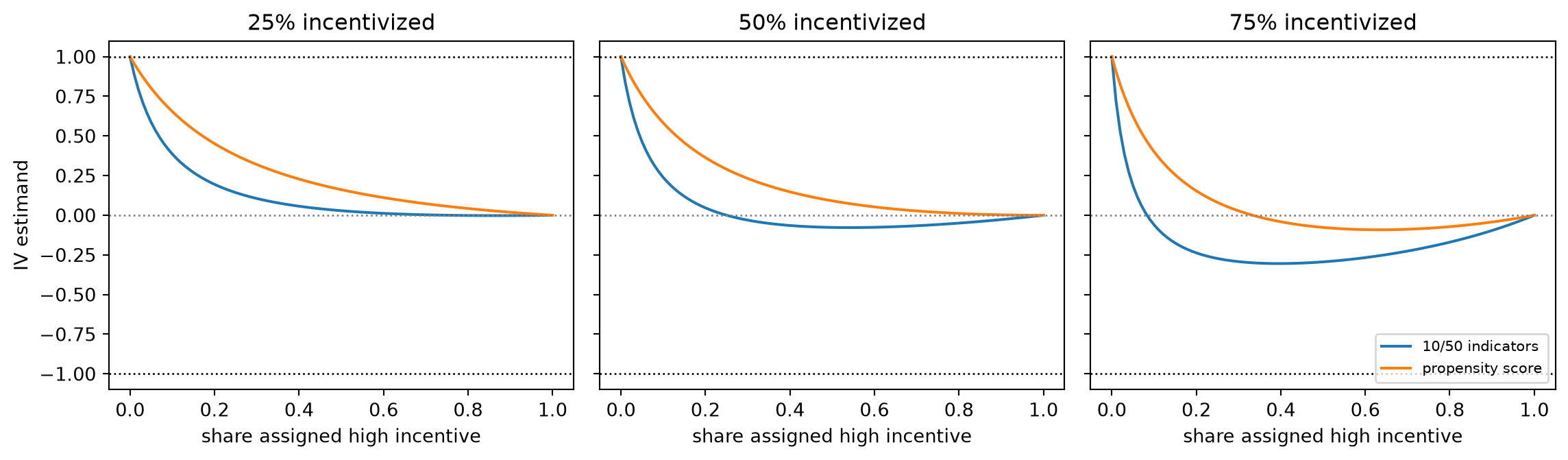

Violations of monotonicity

Without monotonicity, the Wald numerator combines the complier and defier effects with opposite treatment-choice movements. Write LATE for the complier average treatment effect and DATE for the defier average treatment effect. With first stage \(FS=P(CP)-P(DF)\) and observed Wald estimand \(\beta_W\),

\[ \beta_W = \frac{P(CP)LATE - P(DF)DATE}{P(CP)-P(DF)}. \]

Solving for the complier LATE that rationalizes a fixed Wald estimate gives

\[ LATE = \frac{\beta_W + \left(P(DF)/FS\right)DATE} {1 + P(DF)/FS}. \]

def ae_sensitivity_grid() -> pd.DataFrame:
    wald = -0.133
    fs = 0.060
    rows = []
    for prdf in np.arange(0, 0.0601, 0.001):
        for date in np.arange(-0.24, 0.0601, 0.06):
            ratio = prdf / fs
            late = (wald + ratio * date) / (1 + ratio)
            bias = ratio * (late - date)
            rows.append({"prdf": prdf, "date": date, "late": late, "bias": bias})
    return pd.DataFrame(rows)


sens = ae_sensitivity_grid()
sens.head()

	prdf	date	late	bias
0	0.0	-0.24	-0.133	0.0
1	0.0	-0.18	-0.133	0.0
2	0.0	-0.12	-0.133	-0.0
3	0.0	-0.06	-0.133	-0.0
4	0.0	0.00	-0.133	-0.0

fig, ax = plt.subplots(figsize=(7, 4.5))
for date, g in sens.groupby("date"):
    ax.plot(g["prdf"], g["late"], label=f"DATE={date:.2f}")
wald = -0.133
se = 0.026
ax.axhline(wald + 2 * se, color="black", ls=":", lw=1)
ax.axhline(wald - 2 * se, color="black", ls=":", lw=1)
ax.scatter([0], [wald], color="black", zorder=3)
ax.set(xlabel="proportion of defiers", ylabel="LATE rationalizing Wald")
ax.legend(ncol=2, fontsize=8)
plt.show()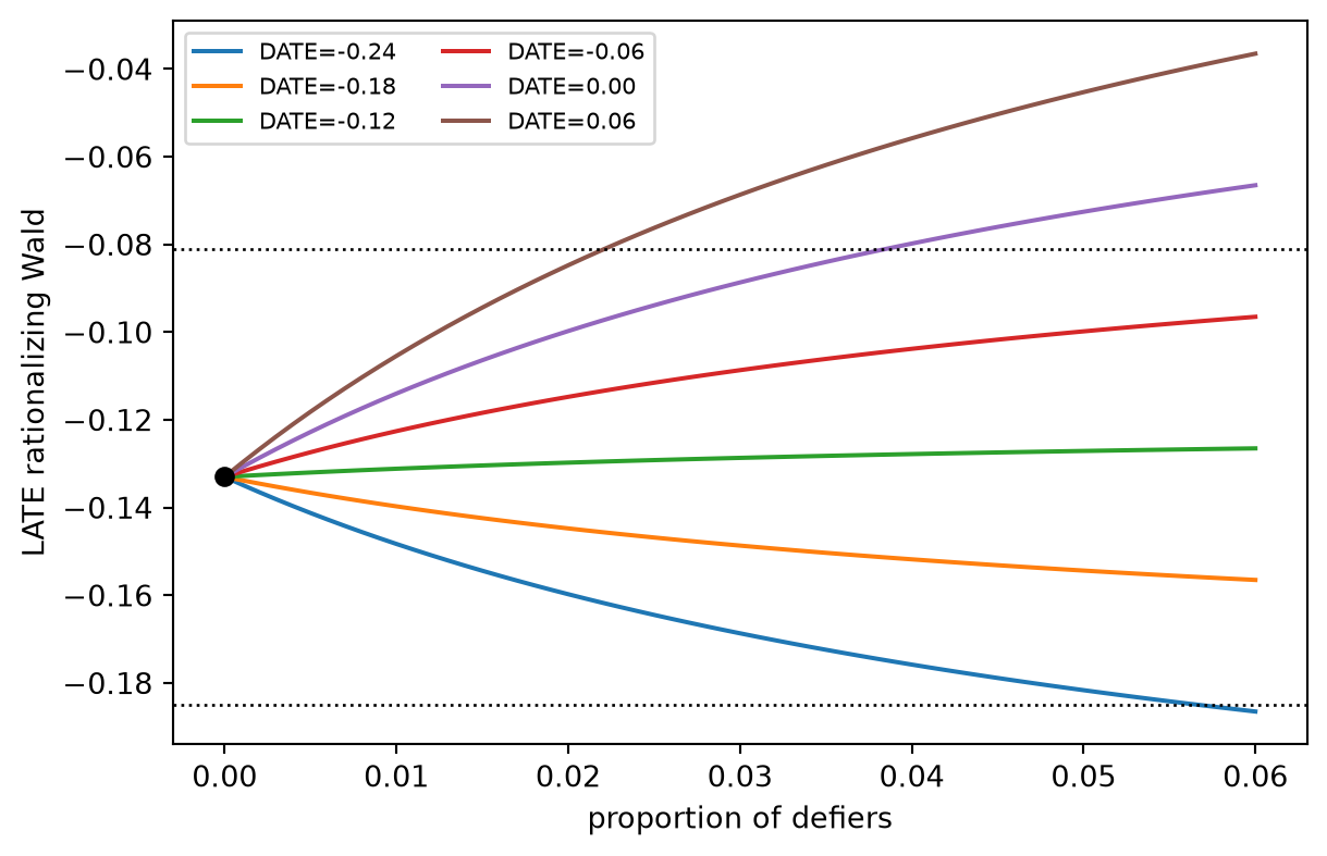

Average monotonicity in judge designs

For many judges, each latent choice group is a vector \(G_i=(D_i(1),\ldots,D_i(J))\). The 2SLS weight for a group is

\[ \omega_{AM}(g) = \sum_{j=1}^J q_j(p_j-\bar p)(g_j-\bar g), \]

where \(q_j=P(Z=j)\), \(p_j=P(D=1\mid Z=j)\), \(\bar p=\sum_jq_jp_j\), and \(\bar g=\sum_jq_jg_j\). Average monotonicity is exactly the claim that the population places no mass on the negatively weighted groups.

def construct_groups(nj: int) -> pd.DataFrame:
    return pd.DataFrame(product([0, 1], repeat=nj), columns=[f"D({j})" for j in range(1, nj + 1)])


def average_monotonicity_df(stevenson: pd.DataFrame) -> pd.DataFrame:
    judge_cols = [c for c in stevenson.columns if c.startswith("judge_pre_")]
    first_stage = pf.feols(
        "jail3 ~ 0 + " + " + ".join(judge_cols),
        data=stevenson,
        vcov="hetero",
    ).coef()
    pscore = np.array([first_stage[c] for c in judge_cols], dtype=float)
    qj = stevenson[judge_cols].mean().to_numpy(dtype=float)
    qj = qj / qj.sum()

    dg = construct_groups(len(judge_cols))
    dvals = dg.to_numpy(dtype=float)
    epj = float(np.sum(qj * pscore))
    dbar = dvals @ qj
    gw = ((pscore - epj) * qj * (dvals - dbar[:, None])).sum(axis=1)
    dg["dbar"] = dbar
    dg["gw"] = gw
    dg["sign"] = np.select([gw < -1e-15, gw > 1e-15], ["Negative", "Positive"], default="Zero")
    return dg


am = average_monotonicity_df(stevenson)
am["sign"].value_counts().to_frame("groups")

	groups
sign
Negative	127
Positive	127
Zero	2

fig, ax = plt.subplots(figsize=(8, 4))
for sign, color in [("Negative", "#d95f02"), ("Positive", "#1b9e77")]:
    ax.hist(am.loc[am["sign"] == sign, "gw"], bins=40, alpha=0.7, label=sign, color=color)
ax.axvline(0, color="black", ls="--", lw=1)
ax.set(xlabel="average-monotonicity group weight", ylabel="number of groups")
ax.legend()
plt.show()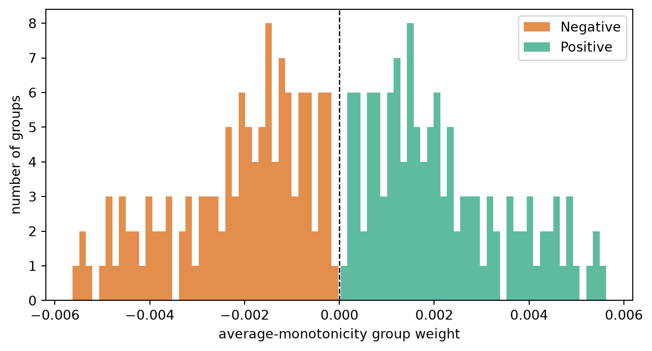

Unordered treatments

For unordered treatments, the treatment states are not a scalar dosage. With three choices and three instrument values, there are \(3^3=27\) response groups. The handbook compares several restrictions:

\[ \text{MON: } 1\{D(j)=j\}\ge 1\{D(k)=j\}\quad\text{for all }j,k, \]

plus extended monotonicity (EM), irrelevance (IR), and next-best (NB). The enumeration is purely logical.

def ch(g: tuple[int, int, int], j: int, k: int) -> int:
    return int(g[k] == j)


def satisfies_mon(g: tuple[int, int, int], dlist: list[int]) -> bool:
    return all(ch(g, j, j) >= ch(g, j, k) for j in dlist for k in dlist)


def satisfies_em(g: tuple[int, int, int]) -> bool:
    return bool((ch(g, 2, 0) == ch(g, 2, 1)) * (ch(g, 1, 2) == ch(g, 1, 0)))


def satisfies_ir(g: tuple[int, int, int], dlist: list[int]) -> bool:
    for k in dlist:
        if ch(g, k, k) == ch(g, k, 0):
            for j in dlist:
                if ch(g, j, k) != ch(g, j, 0):
                    return False
    return True


def satisfies_nb(g: tuple[int, int, int]) -> bool:
    return bool((ch(g, 1, 0) == 0) * (ch(g, 2, 0) == 0))


def unordered_treatment_groups() -> pd.DataFrame:
    dlist = [0, 1, 2]
    rows = []
    for g in product(dlist, repeat=3):
        mon = satisfies_mon(g, dlist)
        em = satisfies_em(g)
        ir = satisfies_ir(g, dlist)
        nb = satisfies_nb(g)
        rows.append(
            {
                "Z0": g[0],
                "Z1": g[1],
                "Z2": g[2],
                "MON": mon,
                "EM": em,
                "IR": ir,
                "NB": nb,
                "KLM": mon and ir and nb,
            }
        )
    return pd.DataFrame(rows).sort_values(["Z2", "Z1", "Z0", "MON"]).reset_index(drop=True)


ug = unordered_treatment_groups()
ug.loc[ug["MON"], ["Z0", "Z1", "Z2", "MON", "EM", "IR", "NB", "KLM"]].reset_index(drop=True)

	Z0	Z1	Z2	MON	EM	IR	NB	KLM
0	0	0	0	True	True	True	True	True
1	0	1	0	True	True	True	True	True
2	0	1	1	True	False	False	True	False
3	1	1	1	True	True	True	False	False
4	0	0	2	True	True	True	True	True
5	0	1	2	True	True	True	True	True
6	1	1	2	True	False	True	False	False
7	2	1	2	True	False	True	False	False
8	0	2	2	True	False	False	True	False
9	2	2	2	True	True	True	False	False

Forward engineering target parameters

The handbook’s second theme is forward engineering: choose the target parameter first and estimate it directly in a model that allows treatment effects to vary.

Propensity weighting for the average causal response

For a binary instrument with covariates, define the instrument propensity score \(q(X)=P(Z=1\mid X)\). A simple weighting estimator for an unconditional LATE/ACR is

\[ \widehat{ACR} = \frac{ \widehat E[Y Z/q(X)]-\widehat E[Y(1-Z)/(1-q(X))] }{ \widehat E[D Z/q(X)]-\widehat E[D(1-Z)/(1-q(X))] }. \]

The Card illustration compares OLS, linear IV, and this propensity-score weighting estimator across the covariate lists used in the R replication. Formulaic constructs the design matrix for the propensity model; scipy optimizes the logit likelihood.

def prep_card(card: pd.DataFrame) -> pd.DataFrame:
    df = card.copy()
    df["Y"] = df["lwage"]
    df["Z"] = df["nearc4"]
    df["D"] = df["educ"]
    interactions = {
        "south_smsa": ("south", "smsa"),
        "south_smsa66": ("south", "smsa66"),
        "smsa_smsa66": ("smsa", "smsa66"),
        "black_exper": ("black", "exper"),
        "black_expersq": ("black", "expersq"),
        "black_south": ("black", "south"),
        "black_smsa": ("black", "smsa"),
        "black_smsa66": ("black", "smsa66"),
        "exper_south": ("exper", "south"),
        "exper_smsa": ("exper", "smsa"),
        "exper_smsa66": ("exper", "smsa66"),
        "expersq_south": ("expersq", "south"),
        "expersq_smsa": ("expersq", "smsa"),
        "expersq_smsa66": ("expersq", "smsa66"),
    }
    for name, (a, b) in interactions.items():
        df[name] = df[a] * df[b]
    return df


def card_covariates(df: pd.DataFrame) -> dict[str, list[str]]:
    reg66 = [c for c in df.columns if c.startswith("reg66")]
    x_geo = ["south", "south66", "smsa", "smsa66", *reg66]
    x_geo_int = [*x_geo, "south_smsa", "south_smsa66", "smsa_smsa66"]
    x_dem = ["black", "exper", "expersq"]
    x_card = [*x_geo, *x_dem]
    x_card_int = [
        *x_card,
        *x_geo_int,
        *[c for c in df.columns if c.startswith("black_")],
        *[c for c in df.columns if c.startswith("exper_")],
        *[c for c in df.columns if c.startswith("expersq_")],
    ]
    return {"NoCov": [], "XGeo": x_geo, "XGeoInt": x_geo_int, "XCard": x_card, "XCardInt": x_card_int}


def controls_rhs(controls: list[str]) -> str:
    return " + ".join(controls) if controls else "1"


def card_ols_iv(df: pd.DataFrame, covs: dict[str, list[str]]) -> pd.DataFrame:
    rows = []
    for name, controls in covs.items():
        ols_formula = "Y ~ D" + (f" + {' + '.join(controls)}" if controls else "")
        rows.append(feols_row(df, ols_formula, "D", "OLS").assign(cov=name))
        iv_formula = f"Y ~ {controls_rhs(controls)} | D ~ Z"
        rows.append(feols_row(df, iv_formula, "D", "Linear IV").assign(cov=name))
    return pd.concat(rows, ignore_index=True)


def qweightlate_est(df: pd.DataFrame, controls: list[str]) -> float:
    q = logit_propensity_formula(f"Z ~ {controls_rhs(controls)}", df)
    z = df["Z"].to_numpy(dtype=float)
    y = df["Y"].to_numpy(dtype=float)
    d = df["D"].to_numpy(dtype=float)
    w1 = z / q
    w0 = (1 - z) / (1 - q)
    return ((y * w1).sum() / w1.sum() - (y * w0).sum() / w0.sum()) / (
        (d * w1).sum() / w1.sum() - (d * w0).sum() / w0.sum()
    )


def qweightlate_table(df: pd.DataFrame, covs: dict[str, list[str]]) -> pd.DataFrame:
    rows = []
    for name, controls in covs.items():
        if not controls:
            continue
        rows.append({"term": "D", "coef": qweightlate_est(df, controls), "se": np.nan, "model": "ACR weighting", "cov": name})
    return pd.DataFrame(rows)


card = prep_card(card_raw)
covs = card_covariates(card)
card_quick = pd.concat([card_ols_iv(card, covs), qweightlate_table(card, covs)], ignore_index=True)
card_quick.pivot_table(index="model", columns="cov", values="coef").loc[
    ["OLS", "Linear IV", "ACR weighting"],
    ["NoCov", "XGeo", "XGeoInt", "XCard", "XCardInt"],
]

cov	NoCov	XGeo	XGeoInt	XCard	XCardInt
model
OLS	0.0521	0.0401	0.0392	0.0747	0.0729
Linear IV	0.1881	0.0906	0.0923	0.1315	0.1326
ACR weighting	NaN	0.0514	0.0408	0.0729	0.0655

The DDML rows in the R replication are intentionally not reproduced here. They are a separate machine-learning translation. The table above keeps the formulas and the estimators that are central to the handbook discussion.

Marginal treatment effects

MTE analysis forward engineers estimators by writing treatment choice as a selection model:

\[ D_i = 1\{P_i \ge U_i\},\qquad P_i = P(D_i=1\mid Z_i,X_i),\qquad U_i\sim U[0,1]. \]

The marginal treatment response functions are

\[ m_d(x,u)=E[Y_i(d)\mid X_i=x,U_i=u], \]

and the marginal treatment effect is

\[ MTE(x,u)=m_1(x,u)-m_0(x,u). \]

If \(m_d(u)\) is approximated by a polynomial basis \(b(u)=(1,u,\ldots,u^K)\), then

\[ m_d(u)=b(u)'\theta_d. \]

Conditioning on observed treatment status integrates over the relevant part of the latent-\(U\) distribution:

\[ E[Y\mid D=1,P=p]= \frac{1}{p}\int_0^p b(u)'\theta_1\,du,\qquad E[Y\mid D=0,P=p]= \frac{1}{1-p}\int_p^1 b(u)'\theta_0\,du. \]

For the monomial \(u^k\),

\[ E[U^k\mid U\le p] = \frac{p^k}{k+1},\qquad E[U^k\mid U>p] = \frac{1-p^{k+1}}{(k+1)(1-p)}. \]

These formulas turn MTR estimation into an ordinary regression with generated regressors. The code below estimates propensity scores by instrument-covariate cells for the simulated tutorial data and then fits the MTR regression with pyfixest.

def cell_propensity(df: pd.DataFrame, d: str, cells: list[str]) -> np.ndarray:
    return df.groupby(cells, observed=True)[d].transform("mean").clip(1e-6, 1 - 1e-6).to_numpy()


def mtr_generated_regressors(df: pd.DataFrame, y: str, d: str, p: np.ndarray, degree: int) -> pd.DataFrame:
    out = df[[y, d]].copy()
    dd = out[d].to_numpy(dtype=float)
    b1 = treated_conditional_basis(p, degree)
    b0 = untreated_conditional_basis(p, degree)
    for k in range(degree + 1):
        out[f"b1_{k}"] = dd * b1[:, k]
        out[f"b0_{k}"] = (1 - dd) * b0[:, k]
    return out


def fit_polynomial_mtr(df: pd.DataFrame, y: str, d: str, p: np.ndarray, degree: int = 2):
    reg = mtr_generated_regressors(df, y, d, p, degree)
    terms = [f"b0_{k}" for k in range(degree + 1)] + [f"b1_{k}" for k in range(degree + 1)]
    fit = pf.feols(f"{y} ~ 0 + " + " + ".join(terms), data=reg, vcov="hetero")
    coefs = fit.coef()
    theta0 = np.array([coefs[f"b0_{k}"] for k in range(degree + 1)], dtype=float)
    theta1 = np.array([coefs[f"b1_{k}"] for k in range(degree + 1)], dtype=float)
    return fit, theta0, theta1


sim["phat_cell"] = cell_propensity(sim, "d", ["z", "x"])
mtr_fit, theta0_hat, theta1_hat = fit_polynomial_mtr(sim, "y", "d", sim["phat_cell"].to_numpy(), degree=2)

pd.DataFrame(
    {
        "term": [f"theta0_{k}" for k in range(3)] + [f"theta1_{k}" for k in range(3)],
        "coef": np.r_[theta0_hat, theta1_hat],
    }
)

	term	coef
0	theta0_0	0.6429
1	theta0_1	0.3273
2	theta0_2	-0.2737
3	theta1_0	0.0908
4	theta1_1	0.4807
5	theta1_2	-0.5954

u_grid = np.linspace(0, 1, 101)
poly = np.column_stack([u_grid**k for k in range(3)])
m0_hat = poly @ theta0_hat
m1_hat = poly @ theta1_hat

fig, ax = plt.subplots(figsize=(7, 4))
ax.plot(u_grid, m0_hat, label="$m_0(u)$")
ax.plot(u_grid, m1_hat, label="$m_1(u)$")
ax.plot(u_grid, m1_hat - m0_hat, label="$MTE(u)$", color="black")
ax.axhline(0, color="gray", lw=0.8)
ax.set(xlabel="$u$", ylabel="response probability / effect", title="Polynomial MTR regression")
ax.legend()
plt.show()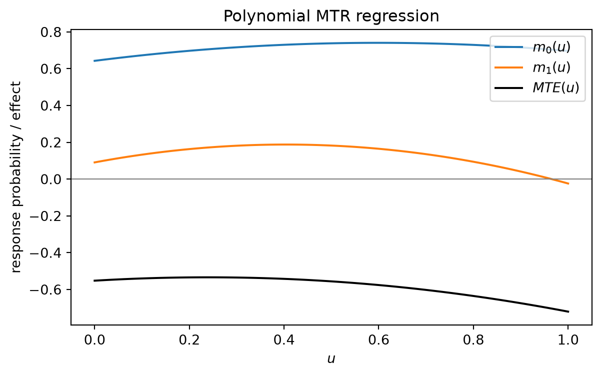

Smooth outcome fits with gamfit

The R ivmte package uses polynomial splines through uSplines(...). In Python, the analogous smooth regression layer here is gamfit. This is not a replacement for the MTR moment program; it is the smooth-regression component one would use when moving from global polynomials to spline-style fits.

ae_smooth_sample = AE.sample(3000, random_state=7).copy()
gam_hours = gamfit.fit(ae_smooth_sample, "hours ~ morekids + s(yob, k=7)", family="gaussian")

smooth_grid = pd.DataFrame(
    {
        "yob": np.tile(np.linspace(AE["yob"].min(), AE["yob"].max(), 80), 2),
        "morekids": np.repeat([0, 1], 80),
    }
)
smooth_grid["pred_hours"] = np.asarray(gam_hours.predict(smooth_grid))

fig, ax = plt.subplots(figsize=(7, 4))
for morekids, g in smooth_grid.groupby("morekids"):
    ax.plot(g["yob"], g["pred_hours"], label=f"morekids={morekids}")
ax.set(xlabel="year of birth", ylabel="fitted hours", title="gamfit smooth of hours on age")
ax.legend()
plt.show()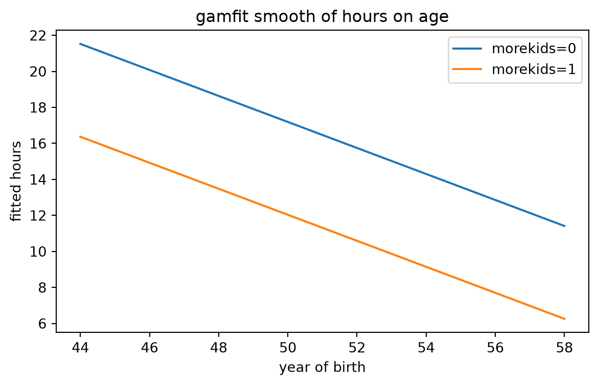

A small scipy MTR-bound program

The ivmte package estimates or bounds target parameters by combining:

1. MTR bases for \(m_0\) and \(m_1\).
2. Moment equations generated by IV-like formulas.
3. Target weights for the estimand of interest.
4. Shape restrictions such as boundedness and monotonicity.

The minimal binary-instrument LP below keeps only the two conditional outcome moments \(E[Y\mid Z=z]\). For each propensity cell \(p_z\),

\[ E[Y\mid Z=z] = \int_{p_z}^1 m_0(u)\,du + \int_0^{p_z}m_1(u)\,du. \]

For a LATE over \([a,b]\), the target is

\[ \frac{1}{b-a}\int_a^b \{m_1(u)-m_0(u)\}\,du. \]

The LP minimizes or maximizes this target subject to the moment equations and bounded MTR functions on a grid.

def moment_row_for_binary_z(p: float, degree: int) -> np.ndarray:
    untreated = power_integral(p, 1, degree)
    treated = power_integral(0, p, degree)
    return np.r_[untreated, treated]


def target_row(interval: tuple[float, float], degree: int) -> np.ndarray:
    a, b = interval
    avg = power_integral(a, b, degree) / (b - a)
    return np.r_[-avg, avg]


@dataclass
class MTEBounds:
    lower: float
    upper: float
    theta_lower: np.ndarray
    theta_upper: np.ndarray
    p0: float
    p1: float
    moments: pd.DataFrame


def binary_z_mte_bounds(
    data: pd.DataFrame,
    y: str,
    d: str,
    z: str,
    degree: int = 2,
    target: str = "late",
    response_bounds: tuple[float, float] = (0.0, 1.0),
    grid_size: int = 101,
    monotone_mte_decreasing: bool = False,
) -> MTEBounds:
    grouped = data.groupby(z, observed=True).agg(p=(d, "mean"), mu=(y, "mean")).reset_index()
    grouped = grouped.sort_values("p").reset_index(drop=True)
    if len(grouped) != 2:
        raise ValueError("This minimal LP expects exactly two propensity-score cells.")

    p0, p1 = map(float, grouped["p"])
    A_eq = np.vstack([moment_row_for_binary_z(p0, degree), moment_row_for_binary_z(p1, degree)])
    b_eq = grouped["mu"].to_numpy(dtype=float)
    c = target_row((p0, p1) if target == "late" else (0, 1), degree)

    u = np.linspace(0, 1, grid_size)
    powers = np.column_stack([u**k for k in range(degree + 1)])
    lower, upper = response_bounds

    A_ub = []
    b_ub = []
    for block in [0, 1]:
        mat = np.zeros((grid_size, 2 * (degree + 1)))
        sl = slice(block * (degree + 1), (block + 1) * (degree + 1))
        mat[:, sl] = powers
        A_ub.append(mat)
        b_ub.append(np.repeat(upper, grid_size))
        A_ub.append(-mat)
        b_ub.append(np.repeat(-lower, grid_size))

    if monotone_mte_decreasing:
        deriv = np.column_stack([np.zeros_like(u)] + [k * u ** (k - 1) for k in range(1, degree + 1)])
        A_ub.append(np.c_[-deriv, deriv])
        b_ub.append(np.zeros(grid_size))

    A_ub = np.vstack(A_ub)
    b_ub = np.concatenate(b_ub)
    lower_res = linprog(c, A_ub=A_ub, b_ub=b_ub, A_eq=A_eq, b_eq=b_eq, method="highs")
    upper_res = linprog(-c, A_ub=A_ub, b_ub=b_ub, A_eq=A_eq, b_eq=b_eq, method="highs")
    if not lower_res.success or not upper_res.success:
        raise RuntimeError((lower_res.message, upper_res.message))

    return MTEBounds(
        lower=float(lower_res.fun),
        upper=float(-upper_res.fun),
        theta_lower=lower_res.x,
        theta_upper=upper_res.x,
        p0=p0,
        p1=p1,
        moments=grouped,
    )


def eval_mte(theta: np.ndarray, degree: int, u: np.ndarray) -> pd.DataFrame:
    n = degree + 1
    powers = np.column_stack([u**k for k in range(n)])
    m0 = powers @ theta[:n]
    m1 = powers @ theta[n:]
    return pd.DataFrame({"u": u, "m0": m0, "m1": m1, "mte": m1 - m0})

ae_late_bounds = binary_z_mte_bounds(AE, y="worked", d="morekids", z="samesex", degree=2, target="late")
ae_ate_bounds = binary_z_mte_bounds(AE, y="worked", d="morekids", z="samesex", degree=2, target="ate")

pd.DataFrame(
    {
        "target": ["LATE over [p0,p1]", "ATE"],
        "p0": [ae_late_bounds.p0, ae_ate_bounds.p0],
        "p1": [ae_late_bounds.p1, ae_ate_bounds.p1],
        "lower": [ae_late_bounds.lower, ae_ate_bounds.lower],
        "upper": [ae_late_bounds.upper, ae_ate_bounds.upper],
    }
)

	target	p0	p1	lower	upper
0	LATE over [p0,p1]	0.3021	0.361	-0.0848	-0.0848
1	ATE	0.3021	0.361	-0.2500	0.0425

curves = pd.concat(
    [
        eval_mte(ae_ate_bounds.theta_lower, 2, u_grid).assign(bound="lower ATE"),
        eval_mte(ae_ate_bounds.theta_upper, 2, u_grid).assign(bound="upper ATE"),
    ],
    ignore_index=True,
)

fig, ax = plt.subplots(figsize=(7, 4))
for label, g in curves.groupby("bound"):
    ax.plot(g["u"], g["mte"], label=label)
ax.axhline(0, color="black", lw=0.8)
ax.set(xlabel="$u$", ylabel="$m_1(u)-m_0(u)$", title="LP-selected MTE curves")
ax.legend()
plt.show()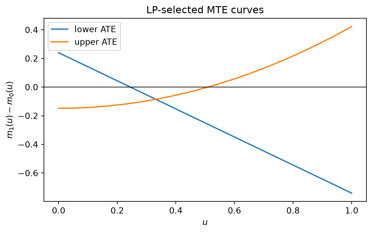

Targets, formulas, and weights in ivmte

The R tutorial’s main call has five conceptual parts:

ivmte(
  data = AE,
  target = "att",
  m0 = ~ u + I(u^2) + yob + u:yob,
  m1 = ~ u + I(u^2) + I(u^3) + yob + u:yob,
  ivlike = worked ~ morekids + samesex + morekids:samesex,
  propensity = morekids ~ samesex + yob
)

The corresponding mathematical pieces are:

• propensity: estimates \(P_i=P(D_i=1\mid Z_i,X_i)\).
• m0, m1: choose bases for \(m_0(x,u)\) and \(m_1(x,u)\).
• ivlike: chooses sample moments, typically linear regression or 2SLS coefficients, that the implied MTR moments must match.
• target: chooses weights \(w_0(x,u),w_1(x,u)\) and reports \(\int w_1m_1-\int w_0m_0\).
• shape restrictions: bound or monotone the admissible MTR/MTE functions.

Formulaic gives the Python analogue of R formula parsing for the observable design matrix:

prop_X = rhs_matrix("morekids ~ samesex + yob", AE)
ivlike_X = rhs_matrix("worked ~ morekids + samesex + morekids:samesex", AE)

pd.DataFrame(
    {
        "formula": ["morekids ~ samesex + yob", "worked ~ morekids + samesex + morekids:samesex"],
        "columns": [", ".join(prop_X.columns), ", ".join(ivlike_X.columns)],
    }
)

	formula	columns
0	morekids ~ samesex + yob	Intercept, samesex, yob
1	worked ~ morekids + samesex + morekids:samesex	Intercept, morekids, samesex, morekids:samesex

The tutorial also discusses custom LATE weights. If \(p_a(x)\) and \(p_b(x)\) are two propensity-score evaluations, the conditional LATE for \(X=x_0\) over \([p_a(x_0),p_b(x_0)]\) uses

\[ w_1(x,u)= \frac{1\{x=x_0\}1\{p_a(x_0)\le u\le p_b(x_0)\}} {P(X=x_0)\{p_b(x_0)-p_a(x_0)\}}, \qquad w_0(x,u)=-w_1(x,u). \]

This is why ivmte target weights are represented as constant splines in \(u\): the computational object is a set of intervals plus multipliers.

Plotting MTRs and weights

In the tutorial, a fitted ivmte object stores the spline dictionary, MTR coefficients, target weights, and IV-like weights. The plotting recipe is:

1. Create a grid for \(u\).
2. Evaluate the MTR basis on the grid.
3. Multiply the basis matrix by the lower-bound or upper-bound coefficients.
4. Plot \(m_0(u)\), \(m_1(u)\), and \(MTE(u)=m_1(u)-m_0(u)\).

The polynomial and LP examples above do exactly that explicitly. The same logic applies to spline bases: replace \((1,u,u^2,\ldots)\) by the chosen spline basis and use gamfit or another basis engine to fit/evaluate the smooth component.

For the weight plot, the core object is a table of intervals:

\[ \{(\ell_r,u_r,\mu_r)\}_{r=1}^R, \]

meaning that observations whose latent \(u\) lies in \([\ell_r,u_r]\) receive multiplier \(\mu_r\). Average weights over a partition are just interval averages of these multipliers. In the binary samesex case, the two propensity scores partition \([0,1]\) into always-taker, complier, and never-taker regions.

p_by_samesex = AE.groupby("samesex", observed=True)["morekids"].mean().sort_values().to_numpy()
weight_regions = pd.DataFrame(
    {
        "region": ["always takers", "same-sex compliers", "never takers"],
        "u_lower": [0, p_by_samesex[0], p_by_samesex[1]],
        "u_upper": [p_by_samesex[0], p_by_samesex[1], 1],
        "treated target weight for LATE": [0, 1 / (p_by_samesex[1] - p_by_samesex[0]), 0],
        "untreated target weight for LATE": [0, -1 / (p_by_samesex[1] - p_by_samesex[0]), 0],
    }
)
weight_regions

	region	u_lower	u_upper	treated target weight for LATE	untreated target weight for LATE
0	always takers	0.0000	0.3021	0.0000	0.0000
1	same-sex compliers	0.3021	0.3610	16.9871	-16.9871
2	never takers	0.3610	1.0000	0.0000	0.0000

Manski-Robins and IV intersection bounds

The Gelbach example uses public-school availability by quarter of birth as an instrument. Without a selection model, one can still bound the potential-outcome means. For a cell with treatment probability \(p_z=P(D=1\mid Z=z)\) and observed mean \(E[Y\mid D=d,Z=z]\), logical outcome bounds \(Y(d)\in[\underline y,\bar y]\) imply

\[ \begin{aligned} E[Y(1)\mid Z=z] &\in \left[ p_zE[Y\mid D=1,Z=z] + (1-p_z)\underline y,\, p_zE[Y\mid D=1,Z=z] + (1-p_z)\bar y \right],\\ E[Y(0)\mid Z=z] &\in \left[ (1-p_z)E[Y\mid D=0,Z=z] + p_z\underline y,\, (1-p_z)E[Y\mid D=0,Z=z] + p_z\bar y \right]. \end{aligned} \]

Intersecting these intervals over instrument values gives IV intersection bounds. Using a constant instrument gives the ordinary Manski-Robins worst-case bounds.

def gelbach_moments(datain: pd.DataFrame, instrument: str = "quarter", treatment: str = "public", outcome: str = "work79") -> pd.DataFrame:
    df = datain.rename(columns={instrument: "z", treatment: "d", outcome: "y"}).copy()
    pscore = df.groupby("z", observed=True)["d"].agg(q=lambda s: len(s) / len(df), p="mean").reset_index()
    means = df.groupby(["z", "d"], observed=True)["y"].mean().reset_index()
    return means.merge(pscore, on="z")


def manski_bounds(moments: pd.DataFrame, ybds: tuple[float, float] = (0.0, 1.0)) -> pd.DataFrame:
    df = moments.sort_values(["d", "p"]).copy()
    ylo, yhi = ybds
    df["lb"] = df["d"] * (df["y"] * df["p"] + ylo * (1 - df["p"])) + (1 - df["d"]) * (
        ylo * df["p"] + df["y"] * (1 - df["p"])
    )
    df["ub"] = df["d"] * (df["y"] * df["p"] + yhi * (1 - df["p"])) + (1 - df["d"]) * (
        yhi * df["p"] + df["y"] * (1 - df["p"])
    )
    inter = df.groupby("d", observed=True).agg(lb=("lb", "max"), ub=("ub", "min")).reset_index()
    ate = pd.DataFrame(
        {
            "d": [np.nan],
            "lb": [inter.loc[inter.d == 1, "lb"].iloc[0] - inter.loc[inter.d == 0, "ub"].iloc[0]],
            "ub": [inter.loc[inter.d == 1, "ub"].iloc[0] - inter.loc[inter.d == 0, "lb"].iloc[0]],
        }
    )
    return pd.concat(
        [df[["z", "d", "p", "lb", "ub"]], inter.assign(z="intersection", p=np.nan), ate.assign(z="ATE", p=np.nan)],
        ignore_index=True,
    )


gelbach_logical = manski_bounds(gelbach_moments(gelbach), ybds=(0, 1))
gelbach_substantive = manski_bounds(gelbach_moments(gelbach), ybds=(0.4, 0.8))
gelbach_const = gelbach.assign(const=1)
worst_case = manski_bounds(gelbach_moments(gelbach_const, instrument="const"), ybds=(0.4, 0.8))

gelbach_out = (
    gelbach_logical[["z", "d", "p", "lb", "ub"]]
    .rename(columns={"lb": "logical_lb", "ub": "logical_ub"})
    .merge(
        gelbach_substantive[["z", "d", "p", "lb", "ub"]].rename(columns={"lb": "substantive_lb", "ub": "substantive_ub"}),
        on=["z", "d", "p"],
        how="outer",
    )
)
gelbach_out.tail(6)

	z	d	p	logical_lb	logical_ub	substantive_lb	substantive_ub
5	3	1.0	0.7930	0.5450	0.7520	0.6278	0.7106
6	4	0.0	0.5532	0.3440	0.8972	0.5653	0.7866
7	4	1.0	0.5532	0.3551	0.8018	0.5338	0.7125
8	ATE	NaN	NaN	-0.2269	0.2521	-0.0979	0.0895
9	intersection	0.0	NaN	0.4958	0.8089	0.6211	0.7463
10	intersection	1.0	NaN	0.5820	0.7479	0.6484	0.7106

worst_case.tail(3).assign(bound_type="substantive worst case")

	z	d	p	lb	ub	bound_type
2	intersection	0.0	NaN	0.5280	0.7810	substantive worst case
3	intersection	1.0	NaN	0.5722	0.7192	substantive worst case
4	ATE	NaN	NaN	-0.2088	0.1912	substantive worst case

What this translation covers

This document now combines the runnable examples with the math objects that generate them:

• Baseline OLS, first-stage, and IV/LATE calculations for Angrist-Evans.
• The ivmte tutorial’s simulated threshold-crossing data.
• Multivalued-instrument 2SLS weights and their dependence on the first-stage specification.
• Monotonicity-violation sensitivity calculations.
• Average-monotonicity weights for the Stevenson judge design.
• Unordered-treatment response-group enumeration.
• Card OLS, linear IV, and propensity-score ACR estimates.
• MTE definitions, polynomial MTR regression, target weights, and a small LP analogue of the ivmte bound program.
• gamfit smooth regression usage for spline-style components.
• Gelbach/Manski-Robins and IV-intersection bounds.

The remaining gap relative to the full R stack is not hidden: a full Python package would still need ivmte’s complete formula language for MTR splines, moment selection, audit-grid iteration, bootstrap confidence regions, specification tests, and solver backends.