---
title: "Choosing an Optimizer for Econometric Estimation"
subtitle: "A comparison of Newton, score, quasi-Newton, trust-region and cubic-regularization methods"
author:
  - Apoorva Lal
  - Krabbs
date: 2026-11-03
jupyter: python3
keep-ipynb: true
execute:
  cache: false
  freeze: false
  warning: false
  error: false
  echo: false
format:
  html:
    theme: cosmo
    toc: true
    toc-depth: 2
    number-sections: true
    html-math-method: katex
    self-contained-math: true
    embed-resources: true
    output-file: index.html
    include-in-header:
      text: |
        <style>
        main{max-width:980px;min-width:0}main a{overflow-wrap:anywhere}
        p{line-height:1.7}.katex-display,.cell-output-display{max-width:100%;overflow-x:auto}
        pre{overflow-x:auto}main img{max-width:100%;height:auto}
        table{font-size:.9rem}figure{margin:1.8rem 0}figcaption{color:#52616b;line-height:1.5}
        h3{margin-top:1.8rem}
        </style>
  typst:
    include-in-header:
      text: |
        #show table: it => block(breakable: false, it)
    output-file: econometric-solvers.pdf
    papersize: a4
    fontsize: 10pt
    margin: {x: 18mm, y: 18mm}
    number-sections: true
---

```{python}
#| include: false
#| code-fold: true
#| code-summary: "Set versions, precision, thread limits, and benchmark constants"
#| output: false
import os
for variable in ["OMP_NUM_THREADS", "OPENBLAS_NUM_THREADS", "MKL_NUM_THREADS",
                 "VECLIB_MAXIMUM_THREADS", "RAYON_NUM_THREADS"]:
    os.environ[variable] = "1"
os.environ["OMP_CANCELLATION"] = "TRUE"
os.environ["OMP_PROC_BIND"] = "TRUE"

from pathlib import Path
from time import perf_counter
import json
import hashlib
import zipfile
from matplotlib.backends.backend_pdf import PdfPages
from matplotlib.lines import Line2D
import platform
import importlib.metadata as metadata
import numpy as np
import pandas as pd
import matplotlib.pyplot as plt
from scipy.special import expit
from scipy.linalg import solve_triangular
from scipy.optimize import minimize, least_squares, linprog
from threadpoolctl import threadpool_limits, threadpool_info
from galahad import tru, arc, qpb
import pyensmallen as pe
import crabbymetrics as cm
from IPython.display import display, Markdown

threadpool_limits(1)
Path("figures").mkdir(exist_ok=True)
FAMILIES = ["OLS", "Ridge", "Logit", "Poisson", "IV-GMM", "NLS", "SCM"]
MAXIT, FW_MAXIT, SECONDS = 1000, 20000, 10.0
SMOOTH = ["GALAHAD TRU", "GALAHAD ARC", "pyensmallen L-BFGS",
          "CrabbyMetrics L-BFGS", "CrabbyMetrics BFGS"]
VERSIONS = {name: metadata.version(name) for name in
            ["galahad-optrove", "pyensmallen", "crabbymetrics", "numpy", "scipy"]}
environment = {
    "versions": VERSIONS, "python": platform.python_version(),
    "platform": platform.platform(), "machine": platform.machine(),
    "cpu": "Apple M4", "memory_bytes": 17179869184,
    "galahad_source_commit": "4275b98e4fdf9af1141d302f04ef944bcda23d32",
    "threads": [{k: v for k, v in info.items() if k != "filepath"}
                for info in threadpool_info()],
    "max_iterations": MAXIT, "fw_max_iterations": FW_MAXIT,
    "callback_time_limit_seconds": SECONDS,
}
Path("environment.json").write_text(json.dumps(environment, indent=2))
WOLFE = [0.9, 0.1]
REFERENCE = ["Ref Newton", "Ref BHHH", "Ref DFP", "Ref BFGS"]
LIKELIHOODS = ["OLS", "Ridge", "Logit", "Poisson", "NLS"]
NATIVE = "CrabbyMetrics native"
NAMES = SMOOTH + REFERENCE + ["GALAHAD QPB", "pyensmallen Frank-Wolfe", NATIVE]
COLORS = dict(zip(NAMES, ["#00838f", "#5bb6ad", "#ba5a18", "#334f96", "#9463a5",
                          "#263238", "#c34242", "#ae8400", "#467a37", "#00838f", "#ba5a18", "#764e20"]))
plt.rcParams.update({"font.size": 9, "axes.spines.top": False, "axes.spines.right": False,
                     "savefig.dpi": 180, "axes.titleweight": "semibold"})
environment.update(reference_wolfe_c2=WOLFE, reference_eigenvalue_floor=1e-5,
                   diagnostic_traces="untimed warm-up; timed fits have logging disabled")
Path("environment.json").write_text(json.dumps(environment, indent=2))
```

```{python}
#| include: false
def make_problem(family, size, level, seed):
    group = 0 if family in ["OLS", "Ridge"] else FAMILIES.index(family)
    rng = np.random.default_rng(20261021 + 100 * group + 10 * size + seed)
    n, p = [(2000, 8), (20000, 24)][size]
    if family == "SCM":
        n, p = [(100, 12), (500, 50)][size]
        factors, loadings = rng.normal(size=(n, 3)), rng.normal(size=(3, p))
        X = factors @ loadings / np.sqrt(3) + [1, .1, .01][level] * rng.normal(size=(n, p))
        beta = np.r_[.2, .3, .5, np.zeros(p - 3)]
        y = X @ beta + .05 * rng.normal(size=n)
        return dict(family=family, X=X, y=y, beta=beta, x0=np.full(p, 1 / p),
                    penalty=np.zeros(p), Z=None)
    features = rng.normal(size=(n, p - 1))
    if family in ["OLS", "Ridge"]:
        Q, _ = np.linalg.qr(features - features.mean(axis=0))
        V, _ = np.linalg.qr(rng.normal(size=(p - 1, p - 1)))
        singular = np.geomspace(1, 1 / [1, 100, 10000][level], p - 1)
        features = np.sqrt(n) * (Q * singular) @ V.T
    X = np.column_stack([np.ones(n), features])
    beta = rng.normal(size=p)
    beta[1:] *= .4 / np.linalg.norm(beta[1:])
    beta[0] = .2
    Z = None
    if family == "Logit":
        beta[1:] *= [1, 4, 12][level] / .4
        y = rng.binomial(1, expit(X @ beta)).astype(float)
    elif family == "Poisson":
        scales = np.r_[1, np.geomspace(1, [1, 100, 10000][level], p - 1)]
        X *= scales
        beta /= scales
        y = rng.poisson(np.exp(X @ beta)).astype(float)
    elif family == "IV-GMM":
        Z = np.column_stack([np.ones(n), rng.normal(size=(n, p + 3))])
        v = rng.normal(size=(n, p - 1))
        strength = np.ones(p - 1)
        strength[0] = [1, .1, .01][level]
        X[:, 1:] = Z[:, 1:p] * strength + v
        y = X @ beta + .7 * v[:, 0] + np.sqrt(1 - .7**2) * rng.normal(size=n)
    elif family == "NLS":
        y = np.exp(X @ beta) + .1 * rng.normal(size=n)
    else:
        y = X @ beta + .25 * rng.normal(size=n)
    penalty = np.r_[0., np.full(p - 1, .01 if family == "Ridge" else 0.)]
    x0 = [0, 4, -6][level] * beta if family == "NLS" else np.zeros(p)
    return dict(family=family, X=np.ascontiguousarray(X), y=y, beta=beta,
                x0=x0, penalty=penalty, Z=Z)
```

```{python}
#| include: false
class Criterion:
    def __init__(self, problem, trace=False, origin=None):
        self.d = problem
        self.kind, self.X, self.y = problem["family"], problem["X"], problem["y"]
        self.n, self.p = self.X.shape
        self.penalty = problem["penalty"]
        self.last = self.value = self.gradient = None
        self.nfg = self.nh = self.nopg = 0
        self.trace = [] if trace else None
        self.origin = perf_counter() if origin is None else origin
        self.scales = np.sqrt(np.mean(self.X**2, axis=0)) if trace else None
        self.deadline = float("inf")
        self.H = None
        if self.kind == "IV-GMM":
            Z = problem["Z"]
            L = np.linalg.cholesky(Z.T @ Z / self.n)
            self.A = solve_triangular(L, Z.T @ self.X / self.n, lower=True)
            self.b = solve_triangular(L, Z.T @ self.y / self.n, lower=True)
        elif self.kind in ["OLS", "Ridge", "SCM"]:
            self.A, self.b = self.X / np.sqrt(self.n), self.y / np.sqrt(self.n)
        if self.kind in ["OLS", "Ridge", "IV-GMM", "SCM"]:
            self.H = self.A.T @ self.A + np.diag(self.penalty)
            self.linear = self.A.T @ self.b
            self.constant = .5 * self.b @ self.b

    @np.errstate(over="ignore", invalid="ignore")
    def fg(self, x):
        if perf_counter() > self.deadline:
            raise TimeoutError("10-second callback budget reached")
        if self.last is None or not np.array_equal(x, self.last):
            self.nfg += 1
            if self.H is not None:
                g = self.H @ x - self.linear
                f = .5 * x @ self.H @ x - self.linear @ x + self.constant
            else:
                eta = self.X @ x
                if self.kind == "Logit":
                    mu = expit(eta)
                    f, residual = np.mean(np.logaddexp(0, eta) - self.y * eta), mu - self.y
                elif self.kind == "Poisson":
                    mu = np.exp(eta)
                    f, residual = np.mean(mu - self.y * eta), mu - self.y
                else:
                    mu = np.exp(eta)
                    f, residual = .5 * np.mean((mu - self.y)**2), mu * (mu - self.y)
                g = self.X.T @ residual / self.n
            self.last, self.value, self.gradient = x.copy(), float(f), g
            if self.trace is not None:
                self.trace.append(dict(evaluation=self.nfg, elapsed=perf_counter() - self.origin,
                                       objective=float(f), scaled_gradient=float(np.max(np.abs(g / self.scales))),
                                       fw_gap=float(g @ x - g.min()) if self.kind == "SCM" else np.nan,
                                       hessian_evaluations=self.nh, opg_evaluations=self.nopg))
        return self.value, self.gradient

    @np.errstate(over="ignore", invalid="ignore")
    def hessian(self, x):
        self.nh += 1
        if self.H is not None:
            return self.H
        eta = self.X @ x
        if self.kind == "Logit":
            mu = expit(eta)
            weights = mu * (1 - mu)
        else:
            mu = np.exp(eta)
            weights = mu if self.kind == "Poisson" else mu * (2 * mu - self.y)
        return self.X.T @ (weights[:, None] * self.X) / self.n

    def fun(self, x):
        return self.fg(x)[0]

    def grad(self, x):
        return self.fg(x)[1]

    def ensmallen(self, x, gradient):
        f, g = self.fg(x)
        gradient[:] = g
        return f

    @np.errstate(over="ignore", invalid="ignore")
    def opg(self, x):
        self.nopg += 1
        eta = self.X @ x
        if self.kind == "Logit":
            scores = (expit(eta) - self.y)[:, None] * self.X
            variance = 1.
        elif self.kind == "Poisson":
            scores = (np.exp(eta) - self.y)[:, None] * self.X
            variance = 1.
        else:
            mu = np.exp(eta) if self.kind == "NLS" else eta
            derivative = mu if self.kind == "NLS" else np.ones(self.n)
            scores = (derivative * (mu - self.y))[:, None] * self.X
            variance = .1**2 if self.kind == "NLS" else .25**2
        return scores.T @ scores / (self.n * variance) + np.diag(self.penalty)
```

```{python}
#| include: false
def strong_wolfe(x, f, g, direction, c2, criterion):
    slope0, calls = float(g @ direction), 0
    assert slope0 < 0

    def evaluate(alpha):
        nonlocal calls
        calls += 1
        ft, gt = criterion.fg(x + alpha * direction)
        return ft, gt, float(gt @ direction)

    def zoom(lo, hi, flo):
        while calls < 40:
            alpha = (lo + hi) / 2
            ft, gt, slope = evaluate(alpha)
            if not np.isfinite(ft + slope) or ft > f + 1e-4 * alpha * slope0 or ft >= flo:
                hi = alpha
            else:
                if abs(slope) <= -c2 * slope0:
                    return alpha, ft, gt
                if slope * (hi - lo) >= 0:
                    hi = lo
                lo, flo = alpha, ft
            if abs(hi - lo) < 1e-16:
                break
        raise RuntimeError("line search failed")

    previous, previous_f, alpha = 0., f, 1.
    while calls < 40:
        ft, gt, slope = evaluate(alpha)
        if (not np.isfinite(ft + slope) or ft > f + 1e-4 * alpha * slope0
                or (calls > 1 and ft >= previous_f)):
            return zoom(previous, alpha, previous_f)
        if abs(slope) <= -c2 * slope0:
            return alpha, ft, gt
        if slope >= 0:
            return zoom(alpha, previous, ft)
        previous, previous_f, alpha = alpha, ft, 2 * alpha
    raise RuntimeError("line search failed")


def inverse_update(M, step, change, method):
    sy = float(step @ change)
    if method == "Ref BFGS":
        A = np.eye(len(step)) - np.outer(step, change) / sy
        updated = A @ M @ A.T + np.outer(step, step) / sy
    else:
        My = M @ change
        updated = M + np.outer(step, step) / sy - np.outer(My, My) / (change @ My)
    return (updated + updated.T) / 2


def solve_reference(d, method, c2, tracing=False):
    start = perf_counter()
    c = Criterion(d, trace=tracing, origin=start)
    prepared = perf_counter()
    c.deadline = start + SECONDS
    x, M = d["x0"].copy(), np.eye(c.p)
    iterations = clipped = skipped = resets = 0
    error, status = "", "iteration limit"
    try:
        f, g = c.fg(x)
        for _ in range(MAXIT):
            if np.max(np.abs(g)) <= 1e-8:
                status = "gradient tolerance"
                break
            if method in ["Ref Newton", "Ref BHHH"]:
                C = c.hessian(x) if method == "Ref Newton" else c.opg(x)
                eigenvalues, Q = np.linalg.eigh(C)
                clipped += int(eigenvalues.min() < 1e-5)
                direction = -Q @ ((Q.T @ g) / np.maximum(eigenvalues, 1e-5))
            else:
                direction = -M @ g
            if not np.all(np.isfinite(direction)) or g @ direction >= 0:
                direction, M = -g, np.eye(c.p)
                resets += 1
            try:
                alpha, fn, gn = strong_wolfe(x, f, g, direction, c2, c)
            except RuntimeError:
                status = "line search failed"
                break
            assert fn <= f + 1e-4 * alpha * float(g @ direction)
            assert abs(float(gn @ direction)) <= c2 * abs(float(g @ direction))
            step, change = alpha * direction, gn - g
            if method in ["Ref DFP", "Ref BFGS"]:
                if step @ change > 1e-12 * np.linalg.norm(step) * np.linalg.norm(change):
                    M = inverse_update(M, step, change, method)
                else:
                    skipped += 1
            x, f, g = x + step, fn, gn
            iterations += 1
        if np.max(np.abs(g)) <= 1e-8:
            status = "gradient tolerance"
    except Exception as exc:
        error, status = str(exc), "exception"
    return x, dict(seconds=perf_counter() - start, preparation_seconds=prepared - start,
                   status=status, iterations=iterations, error=error,
                   fg_evaluations=c.nfg, hessian_evaluations=c.nh, opg_evaluations=c.nopg,
                   clipped=clipped, skipped=skipped, resets=resets), c.trace
```

```{python}
#| include: false
def solve_shared(d, name, tracing=False):
    start = perf_counter()
    c = Criterion(d, trace=tracing, origin=start)
    prepared = perf_counter()
    c.deadline = start + SECONDS
    x = d["x0"].copy()
    status, iterations, error = "returned", np.nan, ""
    module = None
    try:
        if name in ["GALAHAD TRU", "GALAHAD ARC"]:
            module = tru if name.endswith("TRU") else arc
            options = module.initialize()
            options.update(print_level=0, maxit=MAXIT, stop_g_absolute=1e-8,
                           stop_g_relative=0., norm=-1, subproblem_direct=True,
                           clock_time_limit=SECONDS)
            lower = np.tril_indices(c.p)
            ne = len(lower[0])
            module.load(c.p, "dense", ne, None, None, None, options=options)
            x, _ = module.solve(c.p, ne, x, c.fun, c.grad,
                                lambda x: c.hessian(x)[lower])
            info = module.information()
            status, iterations = str(info["status"]), info["iter"]
        elif name == "pyensmallen L-BFGS":
            solver = pe.L_BFGS()
            solver.numBasis, solver.maxIterations = 7, MAXIT
            solver.minGradientNorm, solver.factr = 1e-8, 1e-15
            x = solver.optimize(c.ensmallen, x)
        elif name.startswith("CrabbyMetrics"):
            method = cm.Optimizers.minimize_lbfgs if name.endswith("L-BFGS") else cm.Optimizers.minimize_bfgs
            result = method(c.fun, x, c.grad, max_iterations=MAXIT, tolerance=1e-12)
            x, status, iterations = result["x"], result["message"], result["nit"]
        elif name == "GALAHAD QPB":
            module = qpb
            options = module.initialize()
            options.update(print_level=0, maxit=MAXIT, stop_p=1e-10, stop_d=1e-10, stop_c=1e-10)
            lower = np.tril_indices(c.p)
            ne = len(lower[0])
            module.load(c.p, 1, "dense", ne, None, None, None,
                        "dense", c.p, None, None, None, options)
            x, *_ = module.solve_qp(c.p, 1, c.constant, -c.linear, ne, c.H[lower],
                                   c.p, np.ones(c.p), np.ones(1), np.ones(1),
                                   np.zeros(c.p), np.ones(c.p), x, np.zeros(1), np.zeros(c.p))
            info = module.information()
            status, iterations = str(info["status"]), info["iter"]
        else:
            solver = pe.SimplexFrankWolfe(maxIterations=FW_MAXIT, tolerance=1e-10)
            x = solver.optimize(c.ensmallen, x)
    except Exception as exc:
        error, status = str(exc), "exception"
    finally:
        if module is not None:
            module.terminate()
    return x, dict(seconds=perf_counter() - start, preparation_seconds=prepared - start,
                   status=status, iterations=iterations, error=error,
                   fg_evaluations=c.nfg, hessian_evaluations=c.nh, opg_evaluations=c.nopg), c.trace

def solve_native(d):
    start = perf_counter()
    family, X, y = d["family"], d["X"], d["y"]
    constructors = {
        "OLS": lambda: cm.OLS(), "Ridge": lambda: cm.Ridge(penalty=len(y) * .01),
        "Logit": lambda: cm.Logit(max_iterations=MAXIT, gradient_tolerance=1e-8),
        "Poisson": lambda: cm.Poisson(max_iterations=MAXIT, tolerance=1e-10),
        "IV-GMM": lambda: cm.TwoSLS(), "SCM": lambda: cm.SyntheticControl(max_iterations=MAXIT),
    }
    try:
        model = constructors[family]()
        if family == "SCM":
            model.fit(X, y)
        elif family == "IV-GMM":
            model.fit(X[:, 1:], np.empty((len(y), 0)), d["Z"][:, 1:], y)
        else:
            model.fit(X[:, 1:], y.astype(np.int32) if family == "Logit" else y)
        elapsed = perf_counter() - start
        summary = model.summary()
        x = summary["weights"] if family == "SCM" else np.r_[summary["intercept"], summary["coef"]]
        return x, dict(seconds=elapsed, preparation_seconds=np.nan,
                       iterations=summary.get("iterations", np.nan), status=str(summary.get("converged", "direct solve")),
                       error="", fg_evaluations=np.nan, hessian_evaluations=np.nan, opg_evaluations=np.nan), None
    except Exception as exc:
        return d["x0"].copy(), dict(seconds=perf_counter() - start, preparation_seconds=np.nan,
                                    iterations=np.nan, status="exception", error=str(exc),
                                    fg_evaluations=np.nan, hessian_evaluations=np.nan, opg_evaluations=np.nan), None
```

```{python}
#| include: false
def reference_solution(d):
    c = Criterion(d)
    scales = np.sqrt(np.mean(d["X"]**2, axis=0))
    if d["family"] in ["OLS", "Ridge", "IV-GMM"]:
        A = np.vstack([c.A, np.diag(np.sqrt(d["penalty"]))])
        b = np.r_[c.b, np.zeros(c.p)]
        x = np.linalg.lstsq(A, b, rcond=None)[0]
    elif d["family"] == "SCM":
        result = minimize(c.fun, d["x0"], jac=c.grad, method="SLSQP",
                          bounds=[(0, 1)] * c.p,
                          constraints={"type": "eq", "fun": lambda x: x.sum() - 1,
                                       "jac": lambda x: np.ones(c.p)},
                          options={"ftol": 1e-14, "maxiter": 3000})
        x = result.x
    elif d["family"] == "NLS":
        X, y = d["X"], d["y"]
        fits = [least_squares(lambda x: (np.exp(X @ x) - y) / np.sqrt(c.n), start,
                             jac=lambda x: np.exp(X @ x)[:, None] * X / np.sqrt(c.n),
                             ftol=1e-12, xtol=1e-12, gtol=1e-12, max_nfev=2000)
                for start in [np.zeros(c.p), d["beta"], d["x0"]]]
        x = min(fits, key=lambda fit: np.dot(fit.fun, fit.fun)).x
    else:
        result = minimize(lambda z: c.fun(z / scales), np.zeros(c.p),
                          jac=lambda z: c.grad(z / scales) / scales,
                          hess=lambda z: c.hessian(z / scales) / np.outer(scales, scales),
                          method="trust-exact", options={"gtol": 1e-11, "maxiter": 1000})
        x = result.x / scales
    return x

@np.errstate(over="ignore", invalid="ignore")
def evaluate_solution(d, x, ref):
    c = Criterion(d)
    f, g = c.fg(x)
    fref = c.fun(ref)
    # Score quadratic fits from residuals, independently of the Gram-form callback.
    if c.H is not None:
        residual, reference_residual = c.A @ x - c.b, c.A @ ref - c.b
        f = .5 * (residual @ residual + np.dot(c.penalty, x**2))
        fref = .5 * (reference_residual @ reference_residual + np.dot(c.penalty, ref**2))
        g = c.A.T @ residual + c.penalty * x
    scale = np.sqrt(np.mean(d["X"]**2, axis=0))
    score = np.max(np.abs(g / scale))
    gap = (f - fref) / max(1, abs(fref))
    feasibility = max(0., -float(x.min()), abs(float(x.sum()) - 1)) if c.kind == "SCM" else 0.
    fw_gap = float(g @ x - g.min()) if c.kind == "SCM" else np.nan
    passed = (fw_gap <= 1e-7 and feasibility <= 1e-8) if c.kind == "SCM" else (gap <= 1e-8 and score <= 1e-6)
    passed = bool(passed and np.isfinite(f) and np.isfinite(score) and np.all(np.isfinite(x)))
    eta, eta_ref = d["X"] @ x, d["X"] @ ref
    transform = expit if c.kind == "Logit" else np.exp if c.kind in ["Poisson", "NLS"] else lambda a: a
    pred, predref = transform(eta), transform(eta_ref)
    return dict(objective=f, objective_gap=gap, scaled_gradient=score,
                fw_gap=fw_gap, feasibility=feasibility, accepted=passed,
                coefficient_error=np.linalg.norm(x - ref) / max(1, np.linalg.norm(ref)),
                prediction_error=np.sqrt(np.mean((pred - predref)**2)) / max(1, np.sqrt(np.mean(predref**2))))
```

```{python}
#| include: false
#| code-fold: true
#| code-summary: "Check derivatives and reference fits"
derivative_checks = []
for family in FAMILIES:
    d = make_problem(family, 0, 0, 0)
    c = Criterion(d)
    x = d["beta"].copy()
    step = 1e-5
    directions = np.eye(len(x))
    numeric_g = np.array([(c.fun(x + step * v) - c.fun(x - step * v)) / (2 * step) for v in directions])
    numeric_h = np.column_stack([(c.grad(x + step * v) - c.grad(x - step * v)) / (2 * step) for v in directions])
    g, H = c.grad(x), c.hessian(x)
    ge = np.max(np.abs(g - numeric_g)) / max(1, np.max(np.abs(g)))
    he = np.max(np.abs(H - numeric_h)) / max(1, np.max(np.abs(H)))
    assert ge < 1e-6 and he < 1e-6, (family, ge, he)
    ref = reference_solution(d)
    assert evaluate_solution(d, ref, ref)["accepted"], family
    derivative_checks.append(dict(family=family, gradient_error=ge, hessian_error=he))
display(pd.DataFrame(derivative_checks).style.hide(axis="index").format(
    {"gradient_error": "{:.2e}", "hessian_error": "{:.2e}"}))

# Verify likelihood-score curvature against finite differences of individual losses.
opg_checks = []
for family in LIKELIHOODS:
    d = make_problem(family, 0, 0, 0)
    d = dict(d, X=d["X"][:32], y=d["y"][:32])
    x = d["beta"]
    variance = .1**2 if family == "NLS" else .25**2 if family in ["OLS", "Ridge"] else 1.
    def individual_losses(b):
        eta = d["X"] @ b
        if family == "Logit":
            return np.logaddexp(0, eta) - d["y"] * eta
        if family == "Poisson":
            return np.exp(eta) - d["y"] * eta
        mu = np.exp(eta) if family == "NLS" else eta
        return .5 * (mu - d["y"])**2 / variance
    scores = np.column_stack([(individual_losses(x + 1e-5 * direction) -
                                individual_losses(x - 1e-5 * direction)) / 2e-5
                               for direction in np.eye(len(x))])
    numeric = variance * scores.T @ scores / len(d["y"]) + np.diag(d["penalty"])
    analytic = Criterion(d).opg(x)
    relative = np.max(np.abs(numeric - analytic)) / max(1, np.max(np.abs(analytic)))
    assert relative < 1e-6, (family, relative)
    opg_checks.append(dict(family=family, relative_error=float(relative)))
for method in ["Ref DFP", "Ref BFGS"]:
    M = np.diag([1., 2., 3.])
    step, change = np.array([1., -.5, .2]), np.array([2., -.2, .7])
    updated = inverse_update(M, step, change, method)
    assert np.allclose(updated @ change, step) and np.linalg.eigvalsh(updated).min() > 0

# Full-rank logit designs have finite MLEs if no complete/quasi-separating direction exists.
# Feasibility of S v >= 0 and 1' S v >= 1 would exhibit such a direction.
for size in range(2):
    for level in range(3):
        for seed in range(2):
            d = make_problem("Logit", size, level, seed)
            S = (2 * d["y"] - 1)[:, None] * d["X"]
            check = linprog(np.zeros(S.shape[1]), A_ub=np.vstack([-S, -S.sum(axis=0)]),
                            b_ub=np.r_[np.zeros(len(S)), -1.],
                            bounds=[(None, None)] * S.shape[1], method="highs")
            assert np.linalg.matrix_rank(S) == S.shape[1] and check.status == 2
display(Markdown("**Derivative checks pass for all seven families. All 12 logit samples "
                 "also pass a linear-program check excluding complete or quasi-separation.**"))
```

```{python}
#| include: false
#| code-fold: true
#| code-summary: "Run every method on every applicable instance, with separate diagnostic traces"
#| output: false
def methods_for(family):
    if family == "SCM":
        return [("GALAHAD QPB", "native"), ("pyensmallen Frank-Wolfe", "native"), (NATIVE, "native")]
    methods = [(name, "native") for name in SMOOTH]
    for c2 in WOLFE:
        methods += [(name, f"Wolfe {c2}") for name in REFERENCE
                    if name != "Ref BHHH" or family in LIKELIHOODS]
    if family != "NLS":
        methods += [(NATIVE, "native")]
    return methods

rows, diagnostic_rows, problem_rows, trace_rows, solutions = [], [], [], [], {}
expected_pairs = sum(12 * len(methods_for(family)) for family in FAMILIES)
assert expected_pairs == 1008
for family in FAMILIES:
    for size in range(2):
        for level in range(3):
            for seed in range(2):
                d = make_problem(family, size, level, seed)
                case = f"{family}-{size}-{level}-{seed}"
                ref = reference_solution(d)
                reference_check = evaluate_solution(d, ref, ref)
                assert reference_check["accepted"], (case, reference_check)
                c = Criterion(d)
                H, H0 = c.hessian(ref), c.hessian(d["x0"])
                eigen = np.linalg.eigvalsh(H)
                assert eigen[0] > 0, case
                digest = hashlib.sha256()
                for a in [d["X"], d["y"], d["beta"], d["x0"], d["penalty"], d["Z"]]:
                    if a is not None:
                        digest.update(np.ascontiguousarray(a).tobytes())
                problem_rows.append(dict(case=case, family=family, size=size, level=level, seed=seed,
                                         n=len(d["y"]), p=len(ref), condition=np.linalg.cond(H),
                                         min_eigenvalue=eigen[0], initial_min_eigenvalue=np.linalg.eigvalsh(H0)[0],
                                         reference_objective=c.fun(ref), reference_score=reference_check["scaled_gradient"],
                                         reference_fw_gap=reference_check["fw_gap"], data_sha256=digest.hexdigest()))
                solutions[case + "_reference"] = ref
                methods = methods_for(family)
                for repetition in [-1, 0, 1, 2]:
                    rng = np.random.default_rng(7800 + 100 * size + 10 * level + seed + 1000 * (repetition + 1))
                    for index in rng.permutation(len(methods)):
                        method, setting = methods[index]
                        diagnostic = repetition == -1
                        if method.startswith("Ref "):
                            x, result, history = solve_reference(d, method, float(setting.split()[-1]), diagnostic)
                        elif method == NATIVE:
                            x, result, history = solve_native(d)
                        else:
                            x, result, history = solve_shared(d, method, diagnostic)
                        quality = evaluate_solution(d, x, ref)
                        if result["error"]:
                            quality["accepted"] = False
                        fit_id = f"{case}|{method}|{setting}|{repetition}"
                        row = dict(fit_id=fit_id, case=case, family=family, size=size, level=level, seed=seed,
                                   method=method, setting=setting, repetition=repetition, **result, **quality)
                        solutions[fit_id] = np.asarray(x).copy()
                        if diagnostic:
                            diagnostic_rows.append(row)
                            if history:
                                trace_rows.extend([dict(fit_id=fit_id, case=case, family=family,
                                                        method=method, setting=setting, **point) for point in history])
                        else:
                            rows.append(row)
                    pd.DataFrame(rows).to_csv("results.csv", index=False)
                pd.DataFrame(diagnostic_rows).to_csv("diagnostics.csv", index=False)
                pd.DataFrame(trace_rows).to_csv("traces.csv.gz", index=False, compression="gzip")
                print(f"Completed {case}: {len(rows)}/3024 timed fits", flush=True)
results, problems = pd.DataFrame(rows), pd.DataFrame(problem_rows)
diagnostics, traces = pd.DataFrame(diagnostic_rows), pd.DataFrame(trace_rows)
assert len(results) == 3024 and len(diagnostics) == expected_pairs
problems.to_csv("problems.csv", index=False)
np.savez_compressed("solutions.npz", **solutions)
```

```{python}
#| include: false
def independent_score(d, x, ref):
    X, y, family = d["X"], d["y"], d["family"]
    n = len(y)
    eta, eta_ref = X @ x, X @ ref
    if family in ["OLS", "Ridge", "SCM"]:
        r, rr = eta - y, eta_ref - y
        f = .5 * (r @ r / n + np.dot(d["penalty"], x**2))
        fref = .5 * (rr @ rr / n + np.dot(d["penalty"], ref**2))
        g = X.T @ r / n + d["penalty"] * x
    elif family == "IV-GMM":
        Z = d["Z"]
        moment, ref_moment = Z.T @ (eta - y) / n, Z.T @ (eta_ref - y) / n
        weighted = np.linalg.solve(Z.T @ Z / n, moment)
        f = .5 * moment @ weighted
        fref = .5 * ref_moment @ np.linalg.solve(Z.T @ Z / n, ref_moment)
        g = X.T @ Z @ weighted / n
    else:
        if family == "Logit":
            mu, muref = expit(eta), expit(eta_ref)
            f, fref = np.mean(np.logaddexp(0, eta) - y * eta), np.mean(np.logaddexp(0, eta_ref) - y * eta_ref)
            residual = mu - y
        elif family == "Poisson":
            mu, muref = np.exp(eta), np.exp(eta_ref)
            f, fref = np.mean(mu - y * eta), np.mean(muref - y * eta_ref)
            residual = mu - y
        else:
            mu, muref = np.exp(eta), np.exp(eta_ref)
            f, fref = .5 * np.mean((mu - y)**2), .5 * np.mean((muref - y)**2)
            residual = mu * (mu - y)
        g = X.T @ residual / n
    scaled = float(np.max(np.abs(g) / np.sqrt(np.mean(X**2, axis=0))))
    gap = float((f - fref) / max(1, abs(fref)))
    feasible = max(0., -float(x.min()), abs(float(x.sum()) - 1)) if family == "SCM" else 0.
    fw_gap = float(g @ x - g.min()) if family == "SCM" else np.nan
    passed = (fw_gap <= 1e-7 and feasible <= 1e-8) if family == "SCM" else (gap <= 1e-8 and scaled <= 1e-6)
    return dict(objective=float(f), scaled_gradient=scaled, objective_gap=gap,
                fw_gap=fw_gap, feasibility=feasible,
                accepted=bool(passed and np.isfinite(f) and np.isfinite(scaled) and np.all(np.isfinite(x))))


def recovery(d, x, ref):
    scale = np.sqrt(np.mean(d["X"]**2, axis=0)) if d["family"] != "SCM" else np.ones(len(x))
    transform = expit if d["family"] == "Logit" else np.exp if d["family"] in ["Poisson", "NLS"] else lambda a: a
    pred, truth, predref = [transform(d["X"] @ b) for b in [x, d["beta"], ref]]
    return dict(parameter_rmse=float(np.sqrt(np.mean((scale * (x - d["beta"]))**2))),
                raw_parameter_rmse=float(np.sqrt(np.mean((x - d["beta"])**2))),
                prediction_rmse=float(np.sqrt(np.mean((pred - truth)**2))),
                numerical_parameter_rmse=float(np.sqrt(np.mean((scale * (x - ref))**2))),
                numerical_prediction_rmse=float(np.sqrt(np.mean((pred - predref)**2))))
```

```{python}
#| include: false
#| code-fold: true
#| code-summary: "Independently rescore every timed and diagnostic solution and compute recovery"
#| output: false
audit_rows, recovery_rows, reference_recovery = [], [], []
for problem in problems.to_dict("records"):
    case = problem["case"]
    d = make_problem(problem["family"], problem["size"], problem["level"], problem["seed"])
    ref = solutions[case + "_reference"]
    reference_recovery.append(dict(case=case, family=d["family"], size=problem["size"],
                                   level=problem["level"], seed=problem["seed"], **recovery(d, ref, ref)))
    for frame in [results[results.case == case], diagnostics[diagnostics.case == case]]:
        for row in frame.to_dict("records"):
            x = solutions[row["fit_id"]]
            scored = independent_score(d, x, ref)
            scored["accepted"] = scored["accepted"] and not row["error"]
            assert scored["accepted"] == row["accepted"], (row["fit_id"], scored, row)
            differences = {key: abs(scored[key] - row[key]) for key in ["objective", "scaled_gradient", "objective_gap"]}
            assert differences["objective"] <= 1e-9 * max(1, abs(scored["objective"])), (row["fit_id"], differences)
            assert differences["scaled_gradient"] <= 1e-8 * max(1, scored["scaled_gradient"]), (row["fit_id"], differences)
            audit_rows.append(dict(fit_id=row["fit_id"], repetition=row["repetition"], accepted=scored["accepted"], **differences))
            recovery_rows.append(dict(fit_id=row["fit_id"], case=case, family=d["family"], method=row["method"],
                                      setting=row["setting"], repetition=row["repetition"], level=row["level"],
                                      size=row["size"], seed=row["seed"], accepted=row["accepted"], **recovery(d, x, ref)))
audit = pd.DataFrame(audit_rows)
recoveries = pd.DataFrame(recovery_rows)
reference_recoveries = pd.DataFrame(reference_recovery)
audit.to_csv("independent-audit.csv", index=False)
recoveries.to_csv("recovery.csv", index=False)
reference_recoveries.to_csv("reference-recovery.csv", index=False)
matched_controls = []
for size in range(2):
    for seed in range(2):
        for level in range(3):
            a, b = make_problem("OLS", size, level, seed), make_problem("Ridge", size, level, seed)
            assert np.array_equal(a["X"], b["X"]) and np.array_equal(a["y"], b["y"])
        poisson = [make_problem("Poisson", size, level, seed) for level in range(3)]
        nls = [make_problem("NLS", size, level, seed) for level in range(3)]
        for level in [1, 2]:
            assert np.array_equal(poisson[0]["y"], poisson[level]["y"])
            assert np.allclose(poisson[0]["X"] @ poisson[0]["beta"], poisson[level]["X"] @ poisson[level]["beta"])
            assert np.array_equal(nls[0]["X"], nls[level]["X"]) and np.array_equal(nls[0]["y"], nls[level]["y"])
        matched_controls.append(dict(size=size, seed=seed, passed=True))
validation = dict(instances=len(problems), timed_fits=len(results), diagnostic_fits=len(diagnostics),
                  independent_rescores=len(audit), all_acceptance_decisions_agree=True,
                  matched_controls=matched_controls, derivative_checks=derivative_checks, opg_checks=opg_checks,
                  maximum_objective_difference=float(audit.objective.max()),
                  maximum_scaled_gradient_difference=float(audit.scaled_gradient.max()))
Path("validation.json").write_text(json.dumps(validation, indent=2))
```

```{python}
#| include: false
#| code-fold: true
#| code-summary: "Pair three repetitions per instance without dropping failed runs"
paired = results.groupby(["case", "family", "size", "level", "seed", "method", "setting"], as_index=False).agg(
    accepted=("accepted", "all"), seconds=("seconds", "median"),
    minimum_seconds=("seconds", "min"), maximum_seconds=("seconds", "max"),
    fg_evaluations=("fg_evaluations", "median"), hessian_evaluations=("hessian_evaluations", "median"),
    opg_evaluations=("opg_evaluations", "median"), objective_gap=("objective_gap", "max"),
    scaled_gradient=("scaled_gradient", "max"), fw_gap=("fw_gap", "max"),
    coefficient_error=("coefficient_error", "max"), prediction_error=("prediction_error", "max"))
paired["accepted_ms"] = (1000 * paired.seconds).where(paired.accepted)
summary = paired.groupby(["family", "method", "setting"], as_index=False).agg(
    solved=("accepted", "sum"), attempted=("accepted", "size"),
    median_accepted_ms=("accepted_ms", "median"), worst_gradient=("scaled_gradient", "max"))
paired.to_csv("paired-results.csv", index=False)
summary.to_csv("summary.csv", index=False)
smooth = paired[paired.family != "SCM"]
coverage = smooth.groupby(["method", "setting"], as_index=False).agg(
    solved=("accepted", "sum"), attempted=("accepted", "size"), median_accepted_ms=("accepted_ms", "median"))
display(Markdown(f"**{len(problems)} instances; {len(paired):,} solver–instance–setting combinations; "
                 f"{len(results):,} freshly timed fits and {len(diagnostics):,} diagnostic warm-ups.** "
                 f"{int(results.accepted.sum()):,}/{len(results):,} timed fits pass. An instance is accepted "
                 "for a method and setting only when all three measured repeats pass."))
display(coverage.style.hide(axis="index").format({"median_accepted_ms": "{:.3f}"}))
```

```{python}
#| include: false
#| code-fold: true
#| code-summary: "Plot diagnostic evaluation paths and per-instance recovery"
def save_figure(fig, name):
    fig.savefig(f"figures/{name}.svg", bbox_inches="tight")
    fig.savefig(f"figures/{name}.png", dpi=180, bbox_inches="tight")
    plt.show()
    plt.close(fig)

def convergence_figure(case):
    p = problems.set_index("case").loc[case]
    family, fref = p.family, p.reference_objective
    settings = ["native"] if family == "SCM" else ["Wolfe 0.9", "Wolfe 0.1"]
    fig, axes = plt.subplots(len(settings), 2, figsize=(11.5, 3.5 * len(settings)), squeeze=False,
                             constrained_layout=True)
    for row_index, setting in enumerate(settings):
        eligible = diagnostics[(diagnostics.case == case) & diagnostics.setting.isin([setting, "native"])]
        for _, run in eligible.iterrows():
            points = traces[traces.fit_id == run.fit_id]
            label = run.method.replace("CrabbyMetrics", "CM").replace("pyensmallen", "ens")
            color = COLORS[run.method]
            metric = "fw_gap" if family == "SCM" else "objective"
            if len(points):
                values = points[metric].to_numpy()
                if metric == "objective":
                    values = (values - fref) / max(1, abs(fref))
                values = np.minimum.accumulate(np.where(np.isfinite(values), values, np.inf))
                values = np.maximum(values, 1e-16)
                for ax, axis in zip(axes[row_index], ["evaluation", "elapsed"]):
                    xx = np.maximum(points[axis].to_numpy(), 1e-7)
                    ax.plot(xx, values, color=color, lw=1.6, alpha=.85, label=label)
                # The endpoint is rescored at the returned vector; it is not inferred from best trial values.
                returned_y = run.fw_gap if family == "SCM" else run.objective_gap
                for ax, endx in zip(axes[row_index], [points.evaluation.iloc[-1], run.seconds]):
                    ax.scatter(max(endx, 1e-7), max(returned_y, 1e-16), s=25, edgecolors=color,
                               facecolors=color if run.accepted else "none", zorder=5)
            else:
                # QPB and native estimators expose no callback path: show the genuine returned endpoint only.
                returned_y = run.fw_gap if family == "SCM" else run.objective_gap
                axes[row_index, 1].scatter(max(run.seconds, 1e-7), max(returned_y, 1e-16), s=45,
                                           edgecolors=color, facecolors=color if run.accepted else "none",
                                           marker="D", label=label + " (endpoint)", zorder=6)
        for col_index, ax in enumerate(axes[row_index]):
            ax.set(xscale="log", yscale="log", ylim=(8e-17, None),
                   xlabel="Joint objective/gradient evaluations" if col_index == 0 else "Instrumented warm-up seconds",
                   ylabel="Best evaluated FW gap" if family == "SCM" else "Best evaluated relative objective excess",
                   title=f"{family} · n={int(p.n):,}, p={int(p.p)}, stress {int(p.level)}, seed {int(p.seed)}\n"
                         + ("Native controls" if family == "SCM" else f"Reference {setting}; native controls otherwise"))
            ax.grid(alpha=.2)
            ax.legend(fontsize=7, ncol=3, loc="upper right")
    return fig

def recovery_figure(family):
    frame = recoveries[(recoveries.family == family) & (recoveries.repetition >= 0)]
    frame = frame.groupby(["case", "method", "setting", "level", "size", "seed"], as_index=False).agg(
        accepted=("accepted", "all"), parameter_rmse=("parameter_rmse", "median"),
        prediction_rmse=("prediction_rmse", "median"))
    methods = methods_for(family)
    fig, axes = plt.subplots(1, 2, figsize=(11.5, max(3.8, .42 * (len(methods) + 1))),
                             sharey=True, constrained_layout=True)
    stress_colors = ["#2d70a4", "#bf7915", "#a03b65"]
    for row_index, (method, setting) in enumerate(methods):
        subset = frame[(frame.method == method) & (frame.setting == setting)]
        for _, run in subset.iterrows():
            offset = (run.level - 1) * .19 + (run["size"] - .5) * .07 + (run.seed - .5) * .025
            for ax, metric in zip(axes, ["parameter_rmse", "prediction_rmse"]):
                value = run[metric]
                if np.isfinite(value):
                    ax.scatter(max(value, 1e-12), row_index + offset, s=24,
                               edgecolors=stress_colors[int(run.level)],
                               facecolors=stress_colors[int(run.level)] if run.accepted else "none", linewidths=.9)
    refs = reference_recoveries[reference_recoveries.family == family]
    for _, run in refs.iterrows():
        offset = (run.level - 1) * .19 + (run["size"] - .5) * .07 + (run.seed - .5) * .025
        for ax, metric in zip(axes, ["parameter_rmse", "prediction_rmse"]):
            ax.scatter(max(run[metric], 1e-12), len(methods) + offset, s=23,
                       color=stress_colors[int(run.level)], marker="x")
    labels = [m.replace("CrabbyMetrics", "CM").replace("pyensmallen", "ens") +
              (f" · c₂={s.split()[-1]}" if s.startswith("Wolfe") else "") for m, s in methods] + ["Sample reference"]
    for ax, title in zip(axes, ["Generating-parameter RMSE", "True-mean / structural-prediction RMSE"]):
        ax.set(xscale="log", xlabel=title, title=family, yticks=range(len(labels)), yticklabels=labels)
        ax.grid(axis="x", alpha=.2)
        ax.xaxis.set_minor_formatter(plt.NullFormatter())
    axes[0].invert_yaxis()
    handles = [Line2D([], [], color=c, marker="o", ls="none", label=f"Stress {i}") for i, c in enumerate(stress_colors)]
    handles += [Line2D([], [], color="black", marker="o", markerfacecolor="none", ls="none", label="Rejected"),
                Line2D([], [], color="black", marker="x", ls="none", label="Sample reference")]
    axes[1].legend(handles=handles, fontsize=7, loc="best")
    return fig
```

```{python}
#| include: false
#| label: fig-profile
#| fig-cap: "Runtime profiles across all 72 smooth instances, with failures assigned infinite ratios. BHHH has a separate 60-instance likelihood denominator and is reported in the tables and family figures. Native estimator fits have separate initializers and are excluded."
#| code-fold: true
fig, axes = plt.subplots(1, 2, figsize=(11.5, 4.5), constrained_layout=True)
grid = np.geomspace(1, 300, 400)
for ax, setting in zip(axes, ["Wolfe 0.9", "Wolfe 0.1"]):
    eligible = smooth[(smooth.method.isin(SMOOTH)) | ((smooth.setting == setting) & (smooth.method != "Ref BHHH"))]
    times = eligible.pivot(index="case", columns="method", values="accepted_ms")
    assert len(times) == 72
    ratios = times.div(times.min(axis=1), axis=0).fillna(np.inf)
    for method in SMOOTH + ["Ref Newton", "Ref DFP", "Ref BFGS"]:
        r = ratios[method].to_numpy()
        ax.plot(grid, [(r <= v).mean() for v in grid], color=COLORS[method], lw=1.7,
                label=f"{method} ({np.isfinite(r).sum()}/72)")
    ax.set(xscale="log", xlim=(1, 300), ylim=(0, 1.03), xlabel="Multiple of fastest accepted median time",
           ylabel="Fraction of 72 smooth instances", title=setting)
    ax.grid(alpha=.2)
    ax.legend(fontsize=7, loc="lower right")
save_figure(fig, "performance-profiles")
```

```{python}
#| include: false
#| label: fig-path-ols
#| fig-cap: "OLS: diagnostic evaluation paths for the larger stress-2, seed-0 instance. Native controls are shared across reference Wolfe panels; native estimator and QPB paths are represented by endpoints only."
#| code-fold: true
save_figure(convergence_figure("OLS-1-2-0"), "convergence-ols")
```

```{python}
#| include: false
#| label: fig-recovery-ols
#| fig-cap: "OLS: recovery for every size, stress and seed. Each dot summarizes the three repetitions of its named solver/setting on one instance; open points indicate a rejected instance. Crosses are the independently fitted sample reference."
#| code-fold: true
save_figure(recovery_figure("OLS"), "recovery-ols")
```

```{python}
#| include: false
#| label: fig-path-ridge
#| fig-cap: "Ridge: diagnostic evaluation paths for the larger stress-2, seed-0 instance. Native controls are shared across reference Wolfe panels; native estimator and QPB paths are represented by endpoints only."
#| code-fold: true
save_figure(convergence_figure("Ridge-1-2-0"), "convergence-ridge")
```

```{python}
#| include: false
#| label: fig-recovery-ridge
#| fig-cap: "Ridge: recovery for every size, stress and seed. Each dot summarizes the three repetitions of its named solver/setting on one instance; open points indicate a rejected instance. Crosses are the independently fitted sample reference."
#| code-fold: true
save_figure(recovery_figure("Ridge"), "recovery-ridge")
```

```{python}
#| include: false
#| label: fig-path-logit
#| fig-cap: "Logit: diagnostic evaluation paths for the larger stress-2, seed-0 instance. Native controls are shared across reference Wolfe panels; native estimator and QPB paths are represented by endpoints only."
#| code-fold: true
save_figure(convergence_figure("Logit-1-2-0"), "convergence-logit")
```

```{python}
#| include: false
#| label: fig-recovery-logit
#| fig-cap: "Logit: recovery for every size, stress and seed. Each dot summarizes the three repetitions of its named solver/setting on one instance; open points indicate a rejected instance. Crosses are the independently fitted sample reference."
#| code-fold: true
save_figure(recovery_figure("Logit"), "recovery-logit")
```

```{python}
#| include: false
#| label: fig-path-poisson
#| fig-cap: "Poisson: diagnostic evaluation paths for the larger stress-2, seed-0 instance. Native controls are shared across reference Wolfe panels; native estimator and QPB paths are represented by endpoints only."
#| code-fold: true
save_figure(convergence_figure("Poisson-1-2-0"), "convergence-poisson")
```

```{python}
#| include: false
#| label: fig-recovery-poisson
#| fig-cap: "Poisson: recovery for every size, stress and seed. Each dot summarizes the three repetitions of its named solver/setting on one instance; open points indicate a rejected instance. Crosses are the independently fitted sample reference."
#| code-fold: true
save_figure(recovery_figure("Poisson"), "recovery-poisson")
```

```{python}
#| include: false
#| label: fig-path-ivgmm
#| fig-cap: "IV-GMM: diagnostic evaluation paths for the larger stress-2, seed-0 instance. Native controls are shared across reference Wolfe panels; native estimator and QPB paths are represented by endpoints only."
#| code-fold: true
save_figure(convergence_figure("IV-GMM-1-2-0"), "convergence-iv-gmm")
```

```{python}
#| include: false
#| label: fig-recovery-ivgmm
#| fig-cap: "IV-GMM: recovery for every size, stress and seed. Each dot summarizes the three repetitions of its named solver/setting on one instance; open points indicate a rejected instance. Crosses are the independently fitted sample reference."
#| code-fold: true
save_figure(recovery_figure("IV-GMM"), "recovery-iv-gmm")
```

```{python}
#| include: false
#| label: fig-path-nls
#| fig-cap: "NLS: diagnostic evaluation paths for the larger stress-2, seed-0 instance. Native controls are shared across reference Wolfe panels; native estimator and QPB paths are represented by endpoints only."
#| code-fold: true
save_figure(convergence_figure("NLS-1-2-0"), "convergence-nls")
```

```{python}
#| include: false
#| label: fig-recovery-nls
#| fig-cap: "NLS: recovery for every size, stress and seed. Each dot summarizes the three repetitions of its named solver/setting on one instance; open points indicate a rejected instance. Crosses are the independently fitted sample reference."
#| code-fold: true
save_figure(recovery_figure("NLS"), "recovery-nls")
```

```{python}
#| include: false
#| label: fig-path-scm
#| fig-cap: "SCM: diagnostic evaluation paths for the larger stress-2, seed-0 instance. Native controls are shared across reference Wolfe panels; native estimator and QPB paths are represented by endpoints only."
#| code-fold: true
save_figure(convergence_figure("SCM-1-2-0"), "convergence-scm")
```

```{python}
#| include: false
#| label: fig-recovery-scm
#| fig-cap: "SCM: recovery for every size, stress and seed. Each dot summarizes the three repetitions of its named solver/setting on one instance; open points indicate a rejected instance. Crosses are the independently fitted sample reference."
#| code-fold: true
save_figure(recovery_figure("SCM"), "recovery-scm")
```

```{python}
#| include: false
#| code-fold: true
#| code-summary: "Display all family-level acceptance counts and accepted-time medians"
for family in FAMILIES:
    display(Markdown(f"### {family}"))
    frame = summary[summary.family == family]
    display(frame[["method", "setting", "solved", "attempted", "median_accepted_ms"]]
            .style.hide(axis="index").format({"median_accepted_ms": "{:.3f}"}, na_rep="—"))
```

```{python}
#| include: false
#| code-fold: true
#| code-summary: "Export every instance's diagnostic convergence panel"
#| output: false
with PdfPages("convergence-atlas.pdf") as pdf:
    for case in problems.case:
        fig = convergence_figure(case)
        pdf.savefig(fig)
        plt.close(fig)
```

```{python}
#| include: false
import html
import re

def compact_table(headers, rows):
    assert len(rows) <= 9, "At most ten rows including the header"
    lines = ["| " + " | ".join(headers) + " |", "| " + " | ".join(["---"] * len(headers)) + " |"]
    lines += ["| " + " | ".join(str(v) for v in row) + " |" for row in rows]
    display(Markdown("\n".join(lines)))

def accepted_count(method, setting):
    selected = paired[(paired.family != "SCM") & (paired.method == method) & (paired.setting == setting)]
    return f"{int(selected.accepted.sum())}/{len(selected)}"

def readable_convergence():
    methods = ["GALAHAD TRU", "GALAHAD ARC", "Ref Newton", "Ref BHHH", "Ref BFGS", "pyensmallen L-BFGS"]
    labels = {"GALAHAD TRU": "TRU", "GALAHAD ARC": "ARC", "Ref Newton": "Safeguarded Newton",
              "Ref BHHH": "BHHH", "Ref BFGS": "BFGS", "pyensmallen L-BFGS": "ensmallen L-BFGS"}
    fig, axes = plt.subplots(1, 2, figsize=(10.5, 4.2), constrained_layout=True)
    for ax, family in zip(axes, ["Poisson", "NLS"]):
        case = f"{family}-1-2-0"
        fref = float(problems.set_index("case").loc[case, "reference_objective"])
        for method in methods:
            setting = "Wolfe 0.9" if method.startswith("Ref ") else "native"
            run = diagnostics[(diagnostics.case == case) & (diagnostics.method == method) &
                              (diagnostics.setting == setting)].iloc[0]
            points = traces[traces.fit_id == run.fit_id]
            excess = (points.objective.to_numpy() - fref) / max(1, abs(fref))
            best = np.minimum.accumulate(np.where(np.isfinite(excess), excess, np.inf))
            ax.plot(points.evaluation, np.maximum(best, 1e-16), color=COLORS[method], lw=1.8,
                    label=labels[method])
            ax.scatter(points.evaluation.iloc[-1], max(float(run.objective_gap), 1e-16), s=35,
                       edgecolors=COLORS[method], facecolors=COLORS[method] if run.accepted else "none", zorder=5)
        ax.set(xscale="log", yscale="log", ylim=(7e-17, None), title=family,
               xlabel="Joint objective/gradient evaluations", ylabel="Best evaluated relative objective excess")
        ax.grid(alpha=.2)
    handles, labels = axes[0].get_legend_handles_labels()
    fig.legend(handles, labels, loc="outside lower center", ncol=3, fontsize=8)
    return fig

def readable_recovery():
    selected = [("GALAHAD TRU", "native", "TRU"), ("GALAHAD ARC", "native", "ARC"),
                ("Ref BFGS", "Wolfe 0.9", "BFGS, c₂ = .9"),
                ("pyensmallen L-BFGS", "native", "ensmallen L-BFGS")]
    colors = ["#2d70a4", "#bf7915", "#a03b65"]
    fig, axes = plt.subplots(2, 2, figsize=(10.5, 6.6), constrained_layout=True)
    for axrow, family in zip(axes, ["OLS", "IV-GMM"]):
        frame = recoveries[(recoveries.family == family) & (recoveries.repetition >= 0)]
        per_case = frame.groupby(["case", "method", "setting", "level", "size", "seed"], as_index=False).agg(
            accepted=("accepted", "all"), parameter_rmse=("parameter_rmse", "median"),
            prediction_rmse=("prediction_rmse", "median"))
        for position, (method, setting, _) in enumerate(selected):
            sub = per_case[(per_case.method == method) & (per_case.setting == setting)]
            for _, run in sub.iterrows():
                offset = (run["level"] - 1) * .17 + (run["size"] - .5) * .06 + (run["seed"] - .5) * .025
                for ax, metric in zip(axrow, ["parameter_rmse", "prediction_rmse"]):
                    ax.scatter(max(run[metric], 1e-12), position + offset, s=22,
                               edgecolors=colors[int(run["level"])],
                               facecolors=colors[int(run["level"])] if run["accepted"] else "none")
        for _, run in reference_recoveries[reference_recoveries.family == family].iterrows():
            offset = (run["level"] - 1) * .17 + (run["size"] - .5) * .06 + (run["seed"] - .5) * .025
            for ax, metric in zip(axrow, ["parameter_rmse", "prediction_rmse"]):
                ax.scatter(max(run[metric], 1e-12), len(selected) + offset, s=25,
                           color=colors[int(run["level"])], marker="x")
        labels = [row[2] for row in selected] + ["Sample reference"]
        for ax, xlabel in zip(axrow, ["Generating-parameter RMSE", "True-mean / structural-prediction RMSE"]):
            ax.set(xscale="log", xlabel=xlabel, title=family, yticks=range(len(labels)), yticklabels=labels)
            ax.invert_yaxis()
            ax.xaxis.set_minor_formatter(plt.NullFormatter())
            ax.grid(axis="x", alpha=.2)
    handles = [Line2D([], [], color=c, marker="o", ls="none", label=f"Stress {i}") for i, c in enumerate(colors)]
    handles += [Line2D([], [], color="black", marker="o", markerfacecolor="none", ls="none", label="Rejected"),
                Line2D([], [], color="black", marker="x", ls="none", label="Sample reference")]
    fig.legend(handles=handles, loc="outside lower center", ncol=5, fontsize=8)
    return fig

def supplement_table(frame):
    assert len(frame) <= 9
    return frame.to_html(index=False, border=0, classes="results", na_rep="—", escape=True)

def write_supplement():
    css = """
    :root{font-family:system-ui,sans-serif;color:#20313d;background:#fff;line-height:1.65}
    body{max-width:1100px;margin:0 auto;padding:28px 22px}a{color:#006f87}
    h1,h2,h3{line-height:1.25}h2{margin-top:2.4rem}p{max-width:82ch}
    nav a{display:inline-block;margin-right:1.1em}img{width:100%;height:auto}
    figure{margin:24px 0}figcaption{font-size:.9rem;color:#52616b;max-width:95ch}
    .table-wrap{overflow:auto;max-width:100%}table{border-collapse:collapse;min-width:490px;font-size:.9rem}
    th,td{text-align:left;padding:.4rem .65rem;border-bottom:1px solid #dbe2e5}
    details{margin:16px 0;padding:10px 14px;background:#f5f7f8;border:1px solid #dbe2e5;border-radius:6px}
    summary{cursor:pointer;font-weight:600}pre{overflow:auto;font-size:.82rem;line-height:1.5}
    code{font-family:ui-monospace,monospace}.muted{color:#52616b}h2{scroll-margin-top:1rem}
    """
    sections = ["""<!doctype html><html lang="en"><head><meta charset="utf-8">
    <meta name="viewport" content="width=device-width,initial-scale=1">
    <meta name="robots" content="noindex,nofollow"><title>Econometric Solvers: Detailed Diagnostics and Implementation</title>
    <style>""" + css + """</style></head><body>
    <p><a href="./">Read the paper</a> · <a href="notes.qmd">Executable source</a> ·
    <a href="notes.ipynb">Notebook</a> · <a href="convergence-atlas.pdf">All 84 convergence panels</a></p>
    <h1>Detailed Diagnostics and Implementation</h1>
    <p>This supplement accompanies <em>Choosing an Optimizer for Econometric Estimation</em>.
    It contains the complete family-level results, convergence and recovery figures,
    derivative checks, and executable implementation.</p>
    <nav>""" + "".join(f'<a href="#{f.lower()}">{html.escape(f)}</a>' for f in FAMILIES) +
    '<a href="#implementation">Implementation</a></nav>']
    notes = {
        "OLS": "Collinearity creates nearly flat directions. The SVD reference can recover the sample minimum accurately while the generating coefficients remain poorly estimated.",
        "Ridge": "The same samples as OLS are used. Penalizing slopes improves curvature and introduces shrinkage relative to the unpenalized generating coefficients.",
        "Logit": "Signal increases across stress levels. Every sample has a finite MLE according to the separation check; the test concerns curvature rather than an infinite-coefficient solution.",
        "Poisson": "Only regressor units change across stress levels. Responses and true mean functions are identical, making this a controlled scaling experiment.",
        "IV-GMM": "Weak first stages harm statistical identification. The fixed-weight GMM objective remains a quadratic with the 2SLS minimizer; BHHH is outside this likelihood-free comparison.",
        "NLS": "All stress levels share the same sample, with starts at zero, four times, or minus six times the generating coefficient. The best checked reference is local.",
        "SCM": "All methods enforce nonnegative weights that sum to one. Correlated donors allow weight error and prediction error to move differently."
    }
    for family in FAMILIES:
        sections += [f'<section id="{family.lower()}"><h2>{html.escape(family)}</h2><p>{notes[family]}</p>']
        frame = summary[summary.family == family].copy()
        for title, subset in [("Package APIs", frame[~frame.method.str.startswith("Ref ")]),
                              ("Reference line-search implementations", frame[frame.method.str.startswith("Ref ")])]:
            if subset.empty:
                continue
            table = subset[["method", "setting", "solved", "attempted", "median_accepted_ms"]].copy()
            table["median_accepted_ms"] = table["median_accepted_ms"].map(lambda x: f"{x:.3f}" if np.isfinite(x) else "—")
            table.columns = ["Method", "Step controls", "Passed", "Attempted", "Accepted median (ms)"]
            sections += [f'<h3>{title}</h3><div class="table-wrap">' + supplement_table(table) + '</div>']
        sections += ['<p class="muted">Each family has twelve instances. A pass requires all three timed repeats to satisfy the external criterion. Time medians use accepted instances only and can refer to different subsets.</p>']
        for prefix, caption in [
            ("convergence", "The larger, highest-stress, seed-0 instance. Lines show best evaluated objective values, including trial points; endpoints are rescored at returned vectors. Open endpoints fail the common check. Wall times are instrumented diagnostic warm-ups. QPB and native estimators expose endpoints only."),
            ("recovery", "All twelve size/stress/seed instances. Each point summarizes three timing repetitions for its named method and setting. Open points fail at least one repeat. Colors show stress; crosses show sample-reference recovery. Parameter RMSE uses regressor-RMS units, with unscaled synthetic-control weights; prediction RMSE averages over observations.")]:
            filename = f"{prefix}-{family.lower()}.png"
            sections += [f'<figure><a href="figures/{filename}"><img src="figures/{filename}" loading="lazy" alt="{html.escape(family)} {prefix} diagnostics"></a><figcaption>{caption}</figcaption></figure>']
        sections += ['</section>']
    checks = pd.DataFrame(derivative_checks).copy()
    checks["gradient_error"] = checks.gradient_error.map(lambda x: f"{x:.2e}")
    checks["hessian_error"] = checks.hessian_error.map(lambda x: f"{x:.2e}")
    checks.columns = ["Family", "Gradient finite-difference error", "Hessian finite-difference error"]
    sections += ['<section id="validation"><h2>Numerical checks</h2><p>All 4,032 timed and diagnostic vectors were independently rescored. Acceptance decisions agree for every vector. Likelihood-score finite differences and the DFP/BFGS secant checks also pass.</p><div class="table-wrap">',
                 supplement_table(checks), '</div><p><a href="validation.json">Validation record</a> · <a href="independent-audit.csv">Every rescoring</a> · <a href="verification.json">Build and delivery provenance</a></p></section>']
    sections += ['<section id="implementation"><h2>Executable implementation</h2><p>The source generates all data, references, runs, checks and figures without saved-result inputs or local helper imports. The following panels expose the numerical code; <a href="notes.qmd">the complete Quarto file</a> includes the presentation and export code as well.</p>']
    titles = ["Environment and solver controls", "Matched sample generators", "Criterion, gradient, Hessian and score curvature",
              "Reference Newton, BHHH, DFP and BFGS", "GALAHAD, ensmallen and CrabbyMetrics adapters",
              "Independent references and acceptance targets", "Derivative, score and separation checks",
              "Complete warm-up and timed experiment", "Independent rescoring and recovery definitions",
              "Every returned solution and matched-data checks", "Paired timing summaries"]
    source_cells = re.findall(r'```\{python\}\n(.*?)\n```', Path("notes.qmd").read_text(), re.S)
    for title, code in zip(titles, source_cells[:11]):
        visible = "\n".join(line for line in code.splitlines() if not line.startswith("#|"))
        sections += [f'<details><summary>{html.escape(title)}</summary><pre><code>{html.escape(visible)}</code></pre></details>']
    sections += ['</section><h2>Data and reproduction</h2><p><a href="galahadro-expanded-source.zip">Complete bundle</a> · <a href="results.csv">All timed fits</a> · <a href="recovery.csv">Recovery metrics</a> · <a href="traces.csv.gz">Evaluation traces</a> · <a href="environment.json">Environment</a> · <a href="SHA256SUMS.json">SHA-256 manifest</a></p><p>Install Quarto and uv, then use the bundled source and lockfile:</p><pre><code>uv sync --locked\nQUARTO_PYTHON="$PWD/.venv/bin/python" quarto render notes.qmd --to html</code></pre><p>Package versions are GALAHAD 5.5.3, pyensmallen 0.4.5 and CrabbyMetrics 0.9.1. Measured runs use one CPU thread and float64. The retained notebook supports rendering without another timing run.</p></body></html>']
    Path("supplement.html").write_text("\n".join(sections))
```

::: {.content-visible when-format="html"}
[Read the PDF](econometric-solvers.pdf) · [Detailed diagnostics and implementation](supplement.html)
:::

## Introduction

An econometric estimator is often defined by the criterion it minimizes. Computing
it also requires a choice about curvature, step length and stopping. Those choices
can determine whether a program reaches a useful solution, stops early in a flat
direction, or fails after evaluating an implausibly large trial point. A method
that works well for one likelihood can behave quite differently after changing
the units of a regressor or the starting value.

This experiment compares these choices on seven familiar estimation problems:
OLS, ridge, binary logit, Poisson, linear IV/GMM, nonlinear least squares and
synthetic control. The test set contains **84 simulated instances**, varying sample
size, numerical stress and sample seed. General-purpose solvers share criteria,
starting values and first-derivative callbacks; second-order methods additionally
receive exact Hessians. Existing CrabbyMetrics estimator APIs
provide a separate comparison of complete fitting routines. Every returned vector
is checked independently of its solver's own convergence message.

The strongest result is about **reliability under stress**. GALAHAD's trust-region
and cubic-regularization methods solve every smooth instance to the stated
objective and gradient tolerances. The reference BFGS implementation does so too.
The fastest accepted method varies by problem: safeguarded Newton frequently wins,
and ensmallen L-BFGS is competitive despite receiving no Hessian. BHHH's good
performance on logit and Poisson does not extend to distant starts for nonlinear
least squares. Even among accepted fits, ill-conditioned OLS exposes an important
distinction between accurately fitting the objective and precisely recovering its
coefficients.

The sections below explain the algorithms, describe the experiment, and interpret
the results. The [supplement](supplement.html) contains every family-level table,
all convergence and recovery figures, and the numerical implementation.

## What the optimizers do

Let $f(\beta)$ be the criterion to minimize, $g=\nabla f(\beta)$ its gradient,
and $H=\nabla^2f(\beta)$ its Hessian. Near the current point, the common starting
point is the quadratic approximation

$$q(s)=f(\beta)+g's+\tfrac12s'Hs.$$

The methods differ in how they represent curvature and how they limit the damage
from an inaccurate local approximation.

### Newton: use the observed curvature

Newton solves $Hs=-g$. For a positive-definite Hessian, this is the minimizer
of the quadratic model. Near a well-behaved optimum it can converge rapidly;
for a positive-definite quadratic, the exact unmodified step reaches the optimum
in one iteration. An indefinite Hessian can instead produce an ascent direction,
and a good local direction can still be too long for the nonlinear criterion.

The tested reference implementation is **safeguarded Newton**. It replaces
Hessian eigenvalues below $10^{-5}$ by that floor and uses a line search to
choose how far to move. The floor supplies a descent direction, but changes the
step along flat directions. Its effects matter for the ill-conditioned OLS results;
those results describe this implementation rather than every Newton solver.

### BHHH: estimate curvature from individual scores

BHHH replaces the observed Hessian by an outer product of individual likelihood
scores. For a mean negative log-likelihood, its curvature matrix is
$C=n^{-1}\sum_i s_i s_i'$. The information identity connects this matrix to
expected likelihood curvature at the correctly specified truth. They need not
match in a finite sample or far from the optimum.

This avoids differentiating the score, at the cost of forming a score cross-product
at each step. The reference BHHH implementation uses the same eigenvalue floor
and line search as safeguarded Newton. Gaussian OLS and NLS require the variance
rescaling implied by their squared-error normalization; ridge adds the penalty's
curvature separately. BHHH is used for these likelihood-based problems, logit and
Poisson. Fixed-weight IV/GMM receives no BHHH label.

### DFP and BFGS: learn curvature from successive gradients

Quasi-Newton methods build an inverse-curvature approximation $M$ and use
$d=-Mg$. After moving by $s$, they observe the gradient change $y$ and update
$M$ to satisfy the inverse secant equation $M^+y=s$.

**DFP** updates the inverse approximation directly:

$$M^+=M+\frac{ss'}{s'y}-\frac{Myy'M}{y'My}.$$

**BFGS** uses a different update with the same secant target:

$$M^+=(I-\rho sy')M(I-\rho ys')+\rho ss',\qquad \rho=(s'y)^{-1}.$$

Both retain positive definiteness when the curvature condition $s'y>0$ holds.
The tested implementations start at $M=I$, skip numerically degenerate updates,
and reset a non-descent direction. Their line search is consequential: changing
its curvature requirement materially changes DFP's success rate in this experiment.

### L-BFGS: keep a short curvature history

L-BFGS uses a limited history of step/gradient-change pairs to apply an approximate
inverse Hessian without storing a dense matrix. The tested implementations retain
seven pairs. This is attractive when parameters are numerous or Hessians are
expensive. Here it also provides a useful first-derivative-only comparator at
modest dimension. ensmallen and CrabbyMetrics supply separate implementations
with their own line-search and stopping rules.

### TRU: minimize the quadratic inside a trust region

GALAHAD TRU solves a local step problem of the form

$$\min_{\|s\|\le\Delta}\; g's+\tfrac12s'Hs.$$

The radius $\Delta$ limits the region over which the model is trusted. The
algorithm compares the actual reduction in $f$ with the model's predicted
reduction, accepting useful steps and adjusting the radius. The constraint also
makes the step problem well posed when the Hessian is indefinite.

At a global solution of the Euclidean subproblem, the step obeys
$(H+\lambda I)s=-g$ with $H+\lambda I\succeq0$. Thus the method can change
the direction through a curvature shift, as well as limiting its length. The
benchmark uses exact dense Hessians and direct subproblem solves.

### ARC: penalize long steps with a cubic term

GALAHAD ARC solves a regularized model of the form

$$\min_s\;g's+\tfrac12s'Hs+\tfrac{\sigma}{3}\|s\|^3.$$

The cubic term discourages large steps and dominates negative quadratic
curvature at large distances. Agreement between the model and the evaluated
criterion determines how strongly subsequent steps are regularized. Its step
also satisfies a shifted system, with $\lambda=\sigma\|s\|$ in Euclidean
coordinates. TRU and ARC therefore share an adaptive curvature-shifting mechanism,
while controlling the step through a radius and a penalty, respectively.

### Step acceptance in the reference methods

Reference Newton, BHHH, DFP and BFGS share a strong-Wolfe line search. It asks for
sufficient decrease in the objective and a reduction in the directional slope.
The experiment compares the usual curvature parameter $c_2=.9$ with the stricter
$c_2=.1$. The latter requires a slope closer to zero along the search direction;
it can require more trial evaluations and does not simply mean taking a shorter
step. Package solvers retain their own controls and are timed once per repetition,
without artificial duplication across the two reference settings.

### The constrained synthetic-control methods

Synthetic control minimizes a quadratic over nonnegative donor weights that sum
to one. The comparison therefore uses three constrained methods:

- **GALAHAD QPB** applies a primal–dual interior-point method to the quadratic program.
- **CrabbyMetrics' native solver** uses an active-set method, identifying weights
  on the boundary and solving for the remaining weights.
- **ensmallen Frank–Wolfe** moves toward a simplex vertex chosen from the current
  gradient, using convex combinations to preserve feasibility.

These methods exploit the actual constraint set. The unconstrained smooth
solvers are outside this track. CrabbyMetrics' other native estimators likewise
use their existing fitting routines and initializers; their timing covers a
complete estimator API rather than isolating a generic optimizer.

## Experimental design

Each family has two problem sizes, three stress levels and two sample seeds:
twelve instances per family. The smooth problems use 2,000 or 20,000 observations
and 8 or 24 coefficients, including an intercept. Synthetic control uses 100 or
500 periods and 12 or 50 donors.

| Estimator | Criterion | Stress control |
|:--|:--|:--|
| OLS | Mean squared error | Design singular-value ratio: 1, 100, 10,000 |
| Ridge | Squared error plus slope penalty | Same samples as OLS; penalty 0.01 |
| Logit | Bernoulli negative log-likelihood | Slope norm: 1, 4, 12 |
| Poisson | Poisson negative log-likelihood | Regressor-unit ratio: 1, 100, 10,000 |
| IV/GMM | Fixed-weight quadratic moment criterion | First-stage strength: 1, 0.1, 0.01 |
| Nonlinear least squares | Exponential mean, additive Gaussian error | Starts: zero, $4\beta_0$, $-6\beta_0$ |
| Synthetic control | Squared error on the simplex | Donor noise SD: 1, 0.1, 0.01 |

**Table 1.** Stress has a different meaning in each row. Poisson changes units
while preserving responses and true means. NLS changes starts while preserving
the sample. IV varies identification. Logit samples are checked to exclude
complete or quasi-separation.

There are 1,008 applicable method/instance/setting combinations. Each has one
diagnostic warm-up and three timed repetitions in shuffled order, producing
**3,024 timed fits**. Runs use float64 and one CPU thread on an Apple M4. Timing
includes criterion preparation, solver setup and derivative work, including exact
Hessians where supplied. Diagnostic trace logging is disabled during timed fits.
Native estimator summaries are extracted after timing their fitting calls.

Smooth methods have a 1,000-iteration limit; callback-based fits also have a
ten-second budget. Frank–Wolfe has 20,000 iterations. A successful smooth fit
must have relative objective excess at most $10^{-8}$ and regressor-RMS-scaled
gradient at most $10^{-6}$, using an independent reference. Synthetic control
must have simplex violation at most $10^{-8}$ and a Frank–Wolfe certificate
at most $10^{-7}$. **An instance counts as passed only when all three timed
repetitions meet the external check.** Solver convergence messages are recorded
separately. A small objective/gradient error alone need not ensure precise
coefficients in a flat direction.

## Results

### Reliability depends on the implementation and the problem

TRU, ARC and reference BFGS pass all 72 smooth instances. The remaining methods
show why a single success-rate number requires context: safeguarded Newton's
misses are concentrated in ill-conditioned OLS, while BHHH has difficulty with
distant NLS starts. Stronger Wolfe conditions help DFP substantially.

```{python}
#| echo: false
reliability_rows = []
for method, label in [("Ref Newton", "Safeguarded Newton"), ("Ref BHHH", "BHHH"),
                      ("Ref DFP", "DFP"), ("Ref BFGS", "BFGS (reference)")]:
    reliability_rows.append([label, accepted_count(method, "Wolfe 0.9"), accepted_count(method, "Wolfe 0.1"), "—"])
for method, label in [("GALAHAD TRU", "GALAHAD TRU"), ("GALAHAD ARC", "GALAHAD ARC"),
                      ("pyensmallen L-BFGS", "ensmallen L-BFGS"),
                      ("CrabbyMetrics BFGS", "CrabbyMetrics BFGS"), ("CrabbyMetrics L-BFGS", "CrabbyMetrics L-BFGS")]:
    reliability_rows.append([label, "—", "—", accepted_count(method, "native")])
compact_table(["Method", "Wolfe .9", "Wolfe .1", "Package controls"], reliability_rows)
```

**Table 2.** Passed instances / attempted instances. BHHH's denominator is the
60 likelihood-based instances; the other rows cover 72 smooth instances.
Native estimator APIs are reported separately in the supplement.

BHHH passes every logit and Poisson instance under both settings, but only four
of twelve NLS instances. In the latter model, its score cross-product contains
squared residuals as well as derivatives of the exponential mean. Far from a
good fit, this curvature approximation can differ greatly from the observed
Hessian. Its information-identity motivation provides no uniform guarantee over
these starting points.

For DFP, stricter Wolfe search raises acceptance from 54 to 68 of 72 instances.
NLS improves from four to twelve passes; IV/GMM improves from ten to twelve.
The reference BFGS implementation passes every instance under either setting,
while the existing CrabbyMetrics BFGS call passes 49. The label “BFGS” leaves
important choices about step acceptance, initialization and termination open.
These are comparisons of the stated implementations and tolerances.

### Speed is meaningful only after the accuracy check

@fig-runtime compares each solver with the fastest accepted solver on the *same*
instance. Failed fits receive an infinite time ratio, so an early failure cannot
appear as a speed advantage. The height at ratio one is the fraction of wins;
the eventual height is the fraction of all instances passed.

With reference Wolfe .9, safeguarded Newton is fastest on 34 of the 72 smooth
instances and ensmallen L-BFGS on 25. With Wolfe .1, those counts are 41 and 19.
TRU and ARC provide broader reliability than either of these configurations,
with extra subproblem work. The dimensions here are small enough that forming
and factoring a Hessian can repay its cost through fewer iterations; the same
balance can change at much larger parameter dimension.

![Matched runtime profiles on all 72 smooth instances. Each panel uses one reference Wolfe setting and the same package runs. Failures remain in the denominator. BHHH has a different 60-instance coverage set and is excluded from this profile; native estimator APIs also form a separate track.](figures/performance-profiles.png){#fig-runtime fig-alt="Two matched runtime profiles show speed and reliability across 72 smooth estimation instances."}

### Scaling and distant starts expose different weaknesses

In Poisson, changing regressor units leaves the statistical problem unchanged,
yet ensmallen L-BFGS passes only eight of twelve instances and each generic
CrabbyMetrics method passes four. The reference methods, TRU and ARC pass all
twelve. This is a coordinate-scaling result rather than a deterioration in the
data's information about the mean.

NLS instead holds the observations fixed and changes initialization. TRU, ARC,
safeguarded Newton and reference BFGS pass all twelve instances. ensmallen
L-BFGS passes eleven; the two generic CrabbyMetrics methods pass four each.
@fig-stress-paths shows a difficult starting point alongside the badly scaled Poisson
case. The full timing panels below retain DFP, both Wolfe settings and all package
paths, including failures.

```{python}
#| label: fig-stress-paths
#| fig-cap: "Selected methods on the larger stress-2, seed-0 Poisson and NLS instances (20,000 observations, 24 coefficients). References use Wolfe .9. Lines show the best evaluated objective, including trial points; circles use the returned vector, with open markers indicating rejection. Log-display excess is floored at 1e-16. Evaluation counts exclude the different amounts of curvature work; Figure 1 includes that work in timing."
#| fig-alt: "Convergence paths for badly scaled Poisson and a distant nonlinear-least-squares start; BHHH stalls on the latter while Newton, BFGS, TRU and ARC reach the target."
#| echo: false
save_figure(readable_convergence(), "readable-stress-paths")
```

### Timing and convergence by estimator

The following panels report every estimator family's timing and convergence
paths. Each uses the larger, stress-2, seed-0 instance: 20,000 observations and
24 coefficients for the smooth problems, or 500 periods and 50 donors for
synthetic control. The [84-case atlas](convergence-atlas.pdf) contains every
size, stress and seed.

Within each figure, the left column measures joint objective/gradient evaluations
and the right column measures elapsed time during the instrumented diagnostic
warm-up. Smooth-problem rows use reference Wolfe .9 and .1; the package runs are
shared across rows. Timing tables and @fig-runtime use the separate, uninstrumented
repetitions. Lines include trial points and trace the best evaluated objective.
Circles rescore the returned vector; open markers fail the common accuracy test.
QPB and native estimator APIs expose no callback path, so their time panels show
returned endpoints only.

#### OLS

Collinearity creates flat directions; a small objective error can coexist with slow coefficient adjustment.
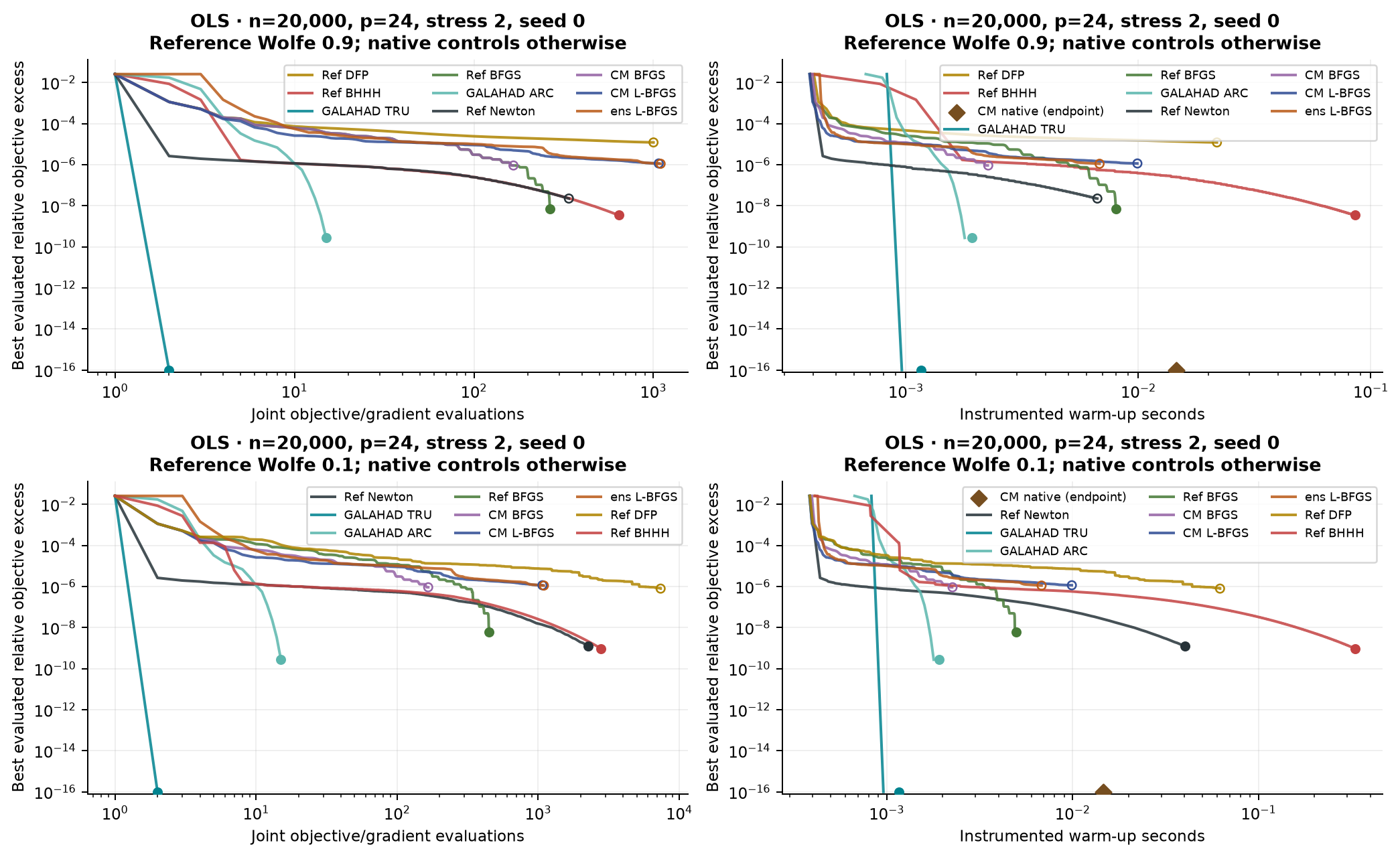
![OLS: relative objective excess against evaluation count (left) and instrumented diagnostic elapsed time (right), with all applicable solvers. Returned endpoints are filled when accepted and open when rejected.](figures/convergence-ols.png){#fig-timing-ols fig-alt="OLS convergence and wall-time panels for all applicable solvers."}

#### Ridge

The slope penalty improves curvature on the same samples used for OLS.
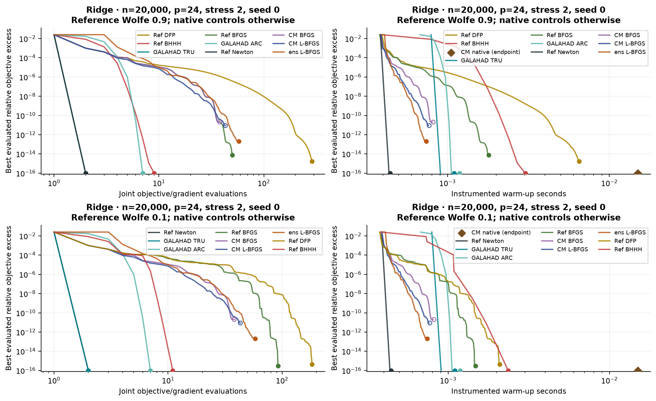
![Ridge: relative objective excess against evaluation count (left) and instrumented diagnostic elapsed time (right), with all applicable solvers. Returned endpoints are filled when accepted and open when rejected.](figures/convergence-ridge.png){#fig-timing-ridge fig-alt="Ridge convergence and wall-time panels for all applicable solvers."}

#### Logit

The strong-signal design weakens likelihood curvature while retaining a finite MLE.
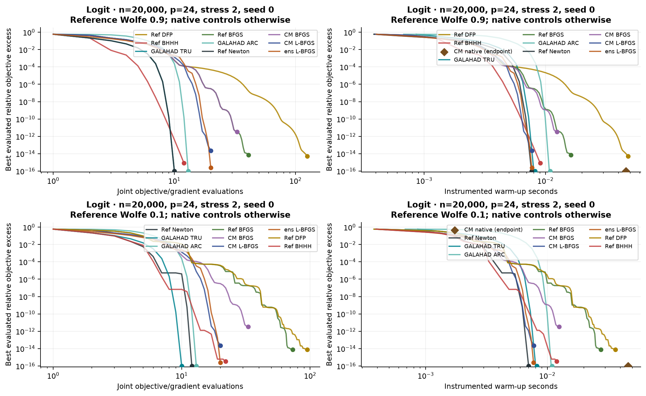
![Logit: relative objective excess against evaluation count (left) and instrumented diagnostic elapsed time (right), with all applicable solvers. Returned endpoints are filled when accepted and open when rejected.](figures/convergence-logit.png){#fig-timing-logit fig-alt="Logit convergence and wall-time panels for all applicable solvers."}

#### Poisson

The highest-stress case changes regressor units while preserving the true mean function.
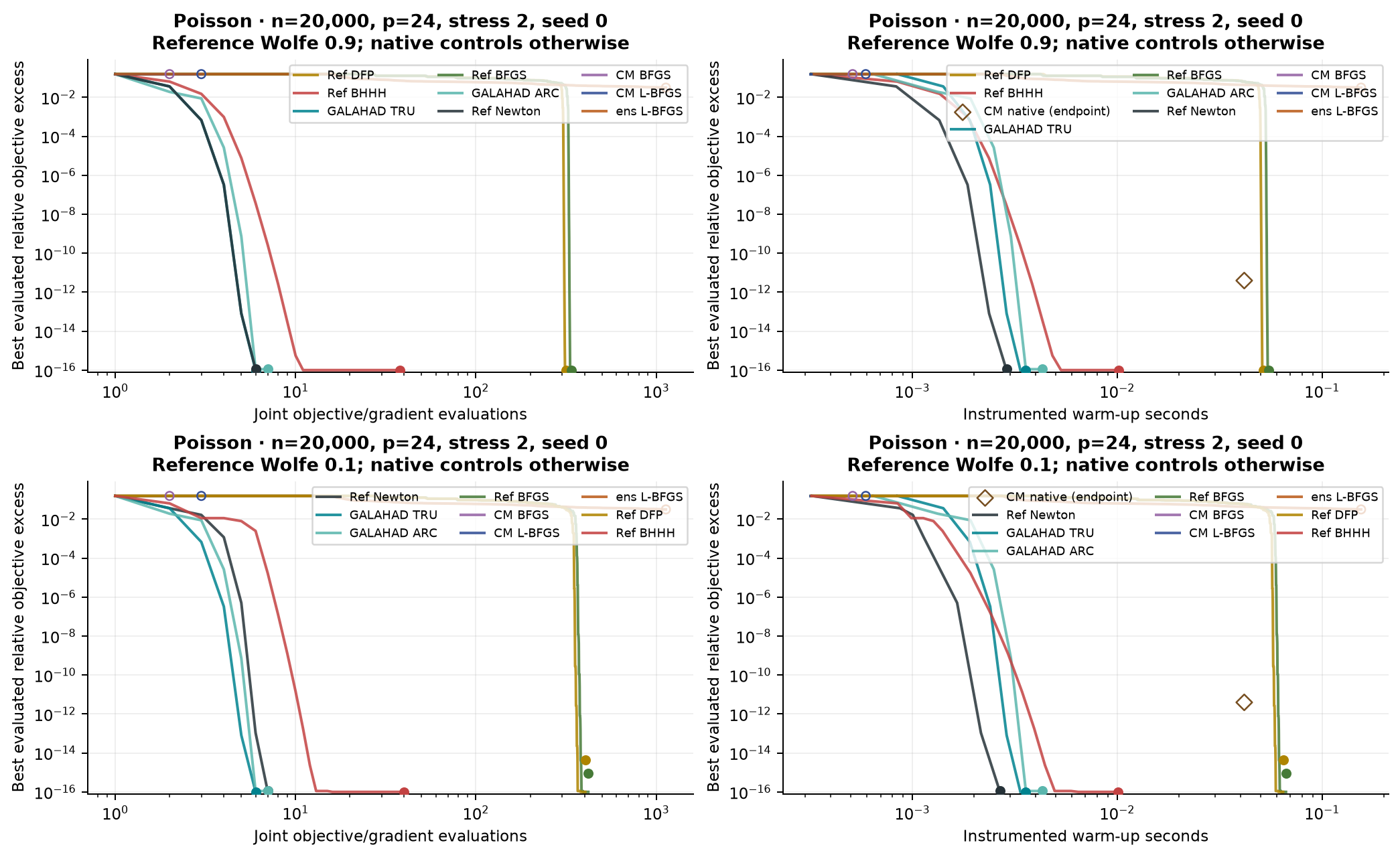
![Poisson: relative objective excess against evaluation count (left) and instrumented diagnostic elapsed time (right), with all applicable solvers. Returned endpoints are filled when accepted and open when rejected.](figures/convergence-poisson.png){#fig-timing-poisson fig-alt="Poisson convergence and wall-time panels for all applicable solvers."}

#### IV/GMM

The weak-first-stage case combines a quadratic sample criterion with limited statistical identification.
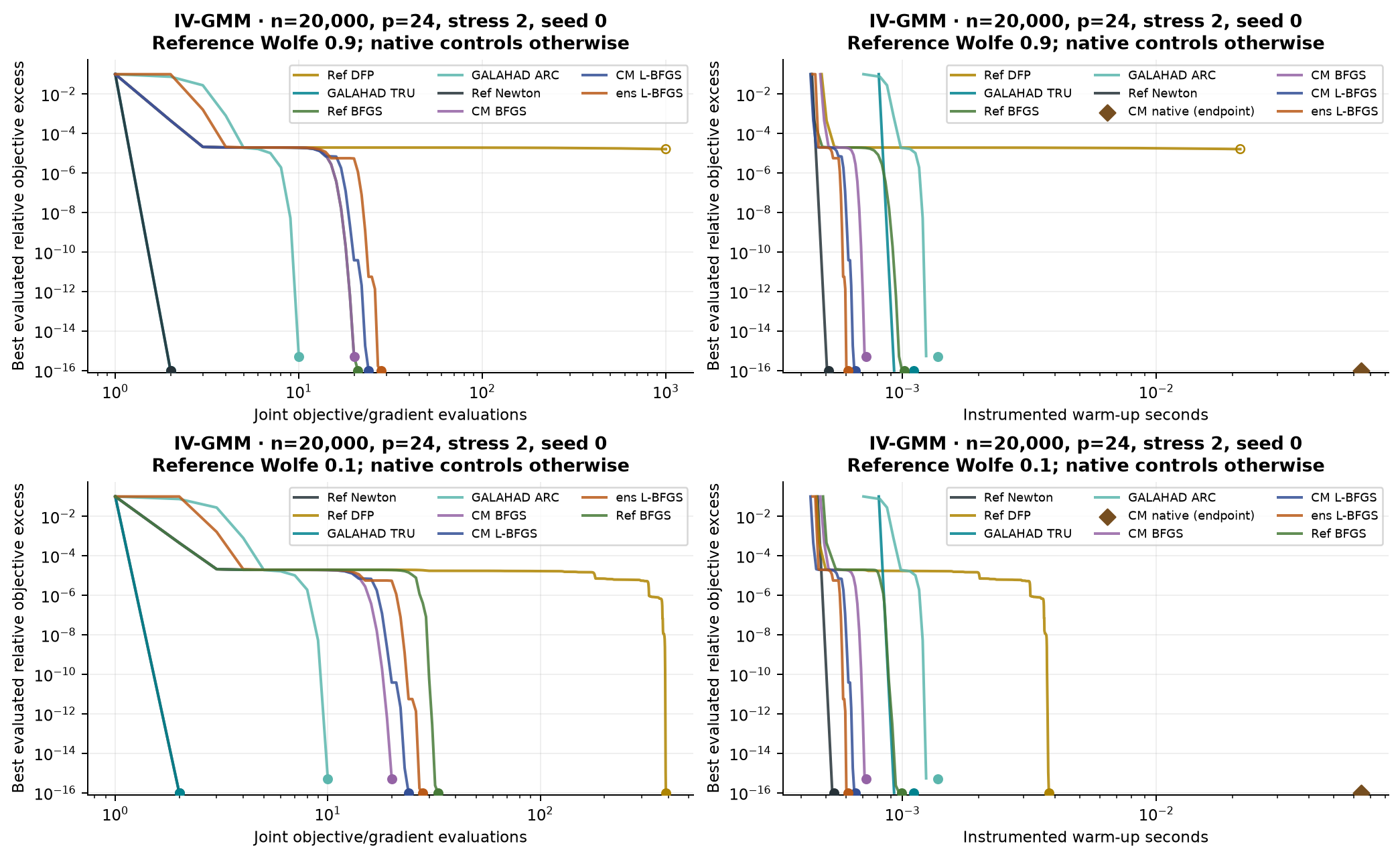
![IV/GMM: relative objective excess against evaluation count (left) and instrumented diagnostic elapsed time (right), with all applicable solvers. Returned endpoints are filled when accepted and open when rejected.](figures/convergence-iv-gmm.png){#fig-timing-ivgmm fig-alt="IV/GMM convergence and wall-time panels for all applicable solvers."}

#### Nonlinear least squares

The distant initial coefficients test step control in the exponential-mean criterion.
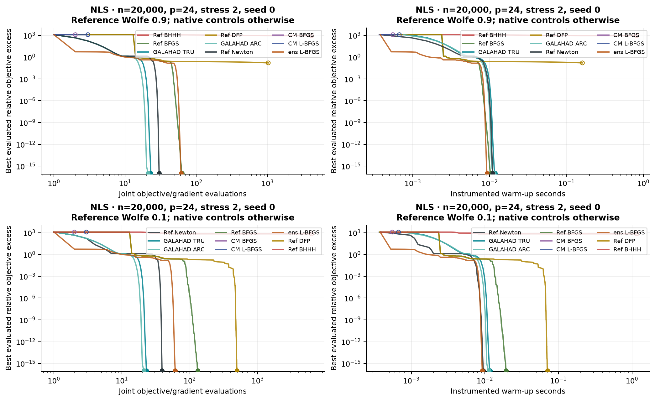
![Nonlinear least squares: relative objective excess against evaluation count (left) and instrumented diagnostic elapsed time (right), with all applicable solvers. Returned endpoints are filled when accepted and open when rejected.](figures/convergence-nls.png){#fig-timing-nls fig-alt="Nonlinear least squares convergence and wall-time panels for all applicable solvers."}

#### Synthetic control

All three methods enforce the simplex; the Frank–Wolfe gap supplies the convergence certificate.
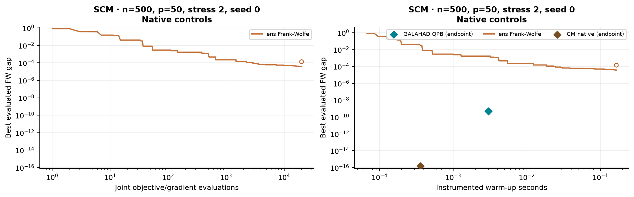
![Synthetic control: Frank–Wolfe gap against evaluation count (left) and instrumented diagnostic elapsed time (right), with all applicable solvers. Returned endpoints are filled when accepted and open when rejected.](figures/convergence-scm.png){#fig-timing-scm fig-alt="Synthetic control convergence and wall-time panels for all applicable solvers."}

### Solving the criterion does not remove identification problems

OLS and ridge clarify the distinction between numerical and statistical
accuracy. All twelve ridge instances pass for the reference methods and both
GALAHAD methods. Without the ridge penalty, collinearity makes a small gradient
compatible with appreciable coefficient disagreement. Among accepted OLS fits,
reference BFGS differs from the SVD coefficients by as much as 13.8% in relative
Euclidean norm, and ARC by 8.8%. Their largest relative prediction disagreements
are only about $1.2\times10^{-4}$ and $9.3\times10^{-5}$, respectively. The
acceptance target controls objectives and gradients; applications requiring
particular coefficients may need a stronger target.

Sampling error is a separate issue. Across the four IV instances at each
strength level, the sample-reference estimate's median raw coefficient RMSE
rises from 0.010 to 0.213 as instruments weaken. An optimizer can closely
reproduce this sample estimate while remaining far from the generating
coefficient. OLS collinearity produces an even sharper coefficient/prediction
contrast. @fig-recovery-reading separates recovery against truth from numerical acceptance.
The full seven-family recovery plots are in the supplement.

```{python}
#| label: fig-recovery-reading
#| fig-cap: "Recovery on all twelve OLS and IV/GMM instances for four representative methods. Each point is one method/setting and size/stress/seed, using the median metric over three timed repeats; open points fail at least one repeat. Colors identify stress and vertical offsets distinguish size/seed. Parameter RMSE averages coefficient errors in regressor-RMS units; prediction RMSE averages over observations. Reference crosses show the sample optimum's statistical error."
#| fig-alt: "OLS and IV recovery panels show coefficient error increasing with collinearity or weak instruments; matching the sample reference does not eliminate this statistical error."
#| echo: false
save_figure(readable_recovery(), "readable-recovery")
```

### Synthetic control rewards specialized constrained solvers

Both QPB and CrabbyMetrics' native active-set solver satisfy the tight simplex
certificate in all twelve instances. The native solver is faster in these small
dense problems. Classic Frank–Wolfe misses the required gap within its fixed
budget, despite preserving feasibility. A method's simplicity and low per-step
cost therefore need to be assessed alongside the accuracy it actually reaches.

```{python}
#| echo: false
simplex_rows = []
for method, label in [("GALAHAD QPB", "GALAHAD QPB"), (NATIVE, "CrabbyMetrics active set"),
                      ("pyensmallen Frank-Wolfe", "ensmallen Frank–Wolfe")]:
    sub = paired[(paired.family == "SCM") & (paired.method == method)]
    simplex_rows.append([label, f"{int(sub.accepted.sum())}/{len(sub)}", f"{1000 * sub.seconds.median():.3f}"])
compact_table(["Method", "Passed", "Median attempted time (ms)"], simplex_rows)
```

**Table 3.** Median time across the twelve instances, after taking the median
of three repetitions within each instance. Failed attempts are included in the
time column; Frank–Wolfe's time is therefore a cost to reach its stopping point,
without achieving the required solution accuracy.

As donor series become more alike, the reference weight RMSE rises while its
prediction RMSE stays small. Several weight vectors can describe nearly the
same fitted path. This is the constrained analogue of the flat-direction
problem in OLS, and is visible in the full recovery diagnostics.

## Implications and limits

For these small-to-moderate dense problems, TRU and ARC are reliable ways to
use exact second derivatives across adverse units and starting points. Reference
BFGS provides the same pass rate using first derivatives, with different timing
and coefficient-accuracy behavior. Safeguarded Newton is often the fastest
accepted method, while its fixed curvature floor merits attention in very flat
problems. BHHH is attractive for some likelihoods, with performance that depends
on the distance from a good fit. DFP illustrates how much a line-search choice
can matter within a single update formula.

A practical choice should specify the software implementation, derivative
information, scaling, starting values and accuracy target together. The existing
CrabbyMetrics wrappers and native estimators are evaluated as supplied; the
experiment makes no changes to their development code. Native estimator calls
include their own preparation and fitting work, so their times do not isolate
an optimizer or programming language.

These conclusions concern the sampled configurations: two seeds, modest dense
parameter dimensions, one CPU thread and analytic derivatives. Large sparse
models, matrix-free Hessian products, stochastic methods, GPUs and statistical
inference are outside the comparison. The NLS reference is the best of three
checked least-squares fits and carries no proof of global optimality. Three
timing repeats are also a small sample, particularly for sub-millisecond fits.

## Technical details and reproduction

The [technical supplement](supplement.html) contains each family's package and
reference tables, complete convergence/recovery figures, numerical checks and
expandable implementation code. The [84-panel atlas](convergence-atlas.pdf) covers every size, stress
and seed rather than only the representative cases shown here.

For a smooth criterion, the two acceptance conditions are

$$\frac{f(\widehat\beta)-f(\widehat\beta_{\mathrm{ref}})}
{\max\{1,|f(\widehat\beta_{\mathrm{ref}})|\}}\le10^{-8},\qquad
\max_j\frac{|\nabla_j f(\widehat\beta)|}{s_j}\le10^{-6},
\quad s_j=\sqrt{n^{-1}\sum_iX_{ij}^2}.$$

For a feasible simplex point, the certificate is
$\nabla f(w)'w-\min_j\nabla_j f(w)\le10^{-7}$; it upper-bounds the convex
objective's suboptimality. Feasibility is checked separately. Gaussian BHHH
curvature is rescaled as $n^{-1}\sum_i r_i^2a_ia_i'/v+P$, where $a_i$ is
the derivative of the mean, $v$ the known simulated noise variance and $P$ the
ridge-penalty Hessian. The noise SD is 0.25 for OLS/ridge and 0.1 for NLS.

OLS, ridge and IV references use augmented SVD least squares; logit and Poisson
use an independent SciPy trust-exact solve in standardized coordinates. All
4,032 timed and diagnostic vectors are independently rescored. NLS uses a
three-start residual-based least-squares reference, and synthetic control a
constrained SLSQP reference with a simplex-gap check.

The [Quarto source](notes.qmd) contains every generator, solver, check, table and
plot; it reads no saved fit results or local helper modules. The
[replication bundle](galahadro-expanded-source.zip) includes the executed
[notebook](notes.ipynb), pinned environment, [timed fits](results.csv),
[paired results](paired-results.csv), [recovery metrics](recovery.csv),
[evaluation traces](traces.csv.gz), [fitted vectors](solutions.npz),
[validation](validation.json) and [SHA-256 manifest](SHA256SUMS.json).

Install Quarto and uv, then run with the bundled source and lockfile:

```sh
uv sync --locked
QUARTO_PYTHON="$PWD/.venv/bin/python" quarto render notes.qmd --to html
```

## References

- Berndt, Hall, Hall and Hausman (1974), “Estimation and Inference in Nonlinear Structural Models.”
- Nocedal and Wright (2006), *Numerical Optimization*, Chapters 4 and 6.
- Cartis, Gould and Toint (2011), “Adaptive Cubic Regularisation Methods for Unconstrained Optimization. Part I.”
- [GALAHAD documentation](https://ralna.github.io/galahad_docs/html/Python/), version 5.5.3.
- [pyensmallen](https://github.com/apoorvalal/pyensmallen), version 0.4.5.
- [CrabbyMetrics](https://apoorvalal.github.io/crabbymetrics/), version 0.9.1.

```{python}
#| include: false
write_supplement()
```
